Project 1: Realistic 3D Projectile Motion
Tip. Every highlighted link in this page is clickable. For fast navagation use Table of Contents
Author: Nels Buhrley
Language: C++17 · Python 3 (visualization)
Build: make — see Build & Run
Snapshot
- Implemented a full 3D projectile simulator in C++17 with drag, Magnus force, and wind rather than idealized no-resistance kinematics.
- Used a 4th-order Runge-Kutta integrator to accurately evolve nonlinear coupled equations of motion.
- Built a Python visualization pipeline for trajectory analysis and comparison across projectile classes and launch parameters.
- Demonstrates core strengths in numerical modeling, physically grounded simulation, and reproducible analysis tooling.
For a fast technical check, jump to Code Structure and Build & Run.
Table of Contents
- Snapshot
- Overview
- Physics Background
- Code Structure
- Results
- Sources of Error
- Build & Run
- Simulation Parameters
- Key Techniques
- Project Structure
Overview
This project implements a 3D projectile motion simulator that goes well beyond the introductory “no air resistance” approximation. The simulation integrates the full equations of motion including aerodynamic drag, spin-induced Magnus force, and environmental wind, producing physically realistic trajectories for projectiles ranging from baseballs to ping-pong balls. Integration is performed with a 4th-order Runge-Kutta scheme, and results are exported to CSV for 3D visualization in Python.
Physics Background
Equations of Motion
A projectile of mass $m$ moving through air at velocity $\vec{v}$ experiences three forces simultaneously:
\[m\vec{a} = \vec{F}_\text{gravity} + \vec{F}_\text{drag} + \vec{F}_\text{Magnus}\]Gravity
\[\vec{F}_\text{gravity} = -mg\hat{z}\]where $g = 9.81$ m/s² is the gravitational acceleration.
Aerodynamic Drag
\[\vec{F}_\text{drag} = -\frac{1}{2}\rho \|\vec{v}_\text{rel}\|^2 C_d A \,\hat{v}_\text{rel}\]where:
- $\rho$ is the air density (default 1.225 kg/m³)
- $\vec{v}\text{rel} = \vec{v} - \vec{v}\text{wind}$ is the velocity relative to the air
- $C_d$ is the drag coefficient (dimensionless)
- $A = \pi r^2$ is the cross-sectional area
- $\hat{v}_\text{rel}$ is the unit vector along the relative velocity
The drag force is proportional to $v^2$ and always opposes the relative motion, producing the characteristic asymmetric trajectory where the descending arc is steeper than the ascending arc.
Magnus Force (Spin Effect)
\[\vec{F}_\text{Magnus} = S\,(\vec{\omega} \times \vec{v})\]where $S$ is the spin factor (units of m²/s) and $\vec{\omega}$ is the angular velocity vector of the projectile. This force arises because a spinning object creates asymmetric pressure distributions in the surrounding airflow — the effect that makes a curveball curve, a golf ball hook or slice, and a table-tennis ball dip.
The direction of the Magnus force is perpendicular to both the spin axis and the velocity, following the right-hand rule of the cross product. For a baseball with backspin ($\vec{\omega}$ horizontal), the Magnus force provides lift; for sidespin, it produces lateral deflection.
Net Acceleration
Combining all forces and dividing by mass:
\[\vec{a} = -g\hat{z} - \frac{\rho \|\vec{v}_\text{rel}\|^2 C_d A}{2m}\hat{v}_\text{rel} + \frac{S}{m}(\vec{\omega} \times \vec{v})\]This is implemented directly in Projectile::calculateAcceleration().
Code Structure
| File | Role |
|---|---|
main.cpp |
Entry point — constructs Run, which handles user interaction |
include/Projectile.h |
Declares Vector3D, Vector4D, Projectile, Trajectory, and preset subclasses |
include/Processing.h |
Declares rk4Simulation(), info helpers, and Run class |
src/Projectile.cpp |
Implements vector operations, calculateAcceleration(), CSV output |
src/Processing.cpp |
Implements RK4 integrator, Run controller with interactive menus |
Preset Projectiles
The code includes physically accurate presets defined as subclasses of Projectile:
| Preset | Mass (kg) | Radius (m) | $C_d$ | Air Density (kg/m³) | Spin Factor $S/m$ | Notes |
|---|---|---|---|---|---|---|
Baseball |
0.149 | 0.0366 | 0.35 | 1.225 | 4.1×10⁻⁴ | Realistic MLB parameters |
pingPongBall |
0.0027 | 0.02 | 0.50 | 1.27 | 0.04 | High spin-to-mass ratio |
perfectProjectile |
1.0 | 0.1 | 0.0 | 0.0 | 0.0 | No drag or spin (textbook parabola) |
RK4 Integration
The 4th-order Runge-Kutta method advances the state vector $\vec{y} = (\vec{r}, \vec{v}, t)$ at each time step:
\[\vec{y}_{n+1} = \vec{y}_n + \frac{h}{6}\left(\vec{k}_1 + 2\vec{k}_2 + 2\vec{k}_3 + \vec{k}_4\right)\]with the standard intermediate evaluations $\vec{k}_1 \ldots \vec{k}_4$. The local truncation error is $\mathcal{O}(h^5)$ and the global error is $\mathcal{O}(h^4)$, providing high accuracy even with moderate time steps.
The simulation terminates when the projectile hits the ground ($z \leq 0$ after launch), and the full trajectory is stored as a sequence of Vector4D points $(x, y, z, t)$.
Results
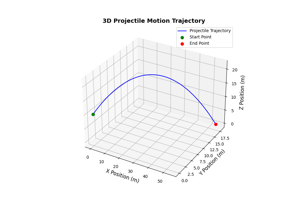
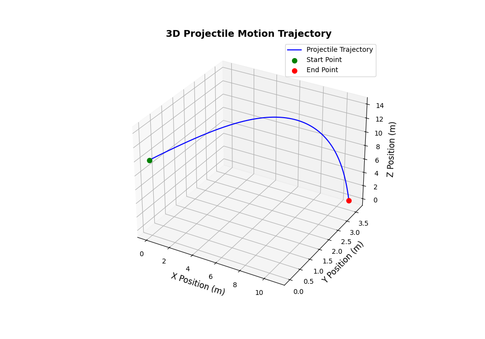
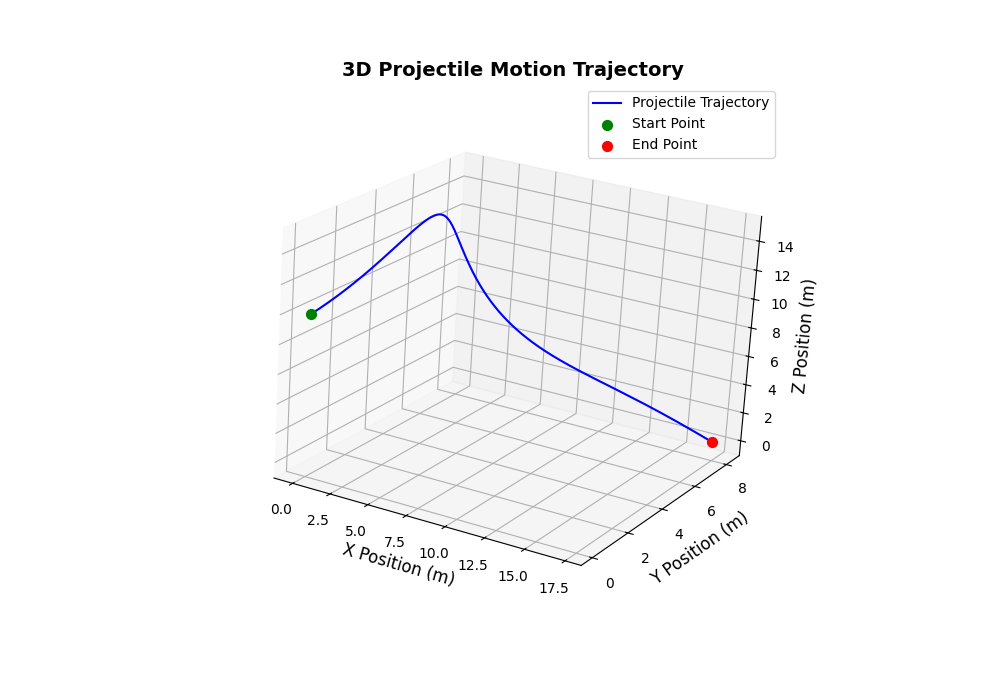
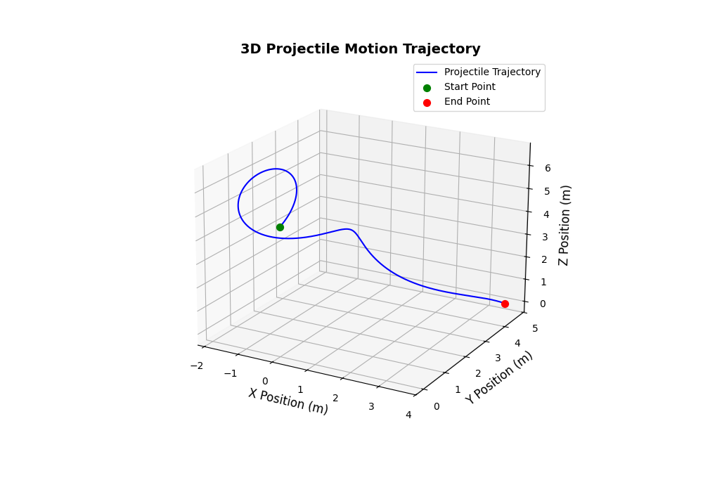
3D trajectory plots showing the effects of drag and Magnus force on projectile paths. Compare the symmetric parabola of the perfectProjectile (no drag) with the asymmetric arcs of the Baseball and pingPongBall (drag + spin).
Sources of Error
| Source | Nature | Mitigation |
|---|---|---|
| Time step truncation | RK4 global error is $\mathcal{O}(h^4)$; too-large $h$ produces inaccurate trajectories | Use small dt (default 0.001 s); validate against analytic parabola |
| Constant drag coefficient | Real $C_d$ varies with Reynolds number (speed) | Adequate for subsonic projectiles; supersonic would need $C_d(\text{Re})$ |
| Fixed air density | Real $\rho$ decreases with altitude ($\rho(h) = \rho_0 e^{-h/H}$) | Negligible for trajectories below ~1 km |
| Rigid-body assumption | Spin rate assumed constant throughout flight | Acceptable for short flights; longer trajectories need spin decay |
| Ground model | Flat ground at $z = 0$; no terrain | Sufficient for ballistics validation |
Build & Run
Prerequisites
- C++17 compatible compiler (
clang++org++) - Python 3 with
pandasandmatplotlib
Build
make
Run
./bin/main
The program presents an interactive menu to choose between validation runs, preset projectiles, or custom parameters. Output is written to Output/trajectoryN.csv (auto-incrementing filenames).
Visualize
python3 ploting.py
Produces a 3D trajectory plot saved to Output/trajectoryN.png.
Simulation Parameters
Configured interactively at runtime or via preset classes:
| Parameter | Description | Units |
|---|---|---|
| Initial position | Launch point $(x_0, y_0, z_0)$ | m |
| Initial velocity | Launch velocity $(v_x, v_y, v_z)$ | m/s |
| Spin vector | Angular velocity $(\omega_x, \omega_y, \omega_z)$ | rad/s |
| Mass | Projectile mass | kg |
| Radius | Projectile radius (for drag area $A = \pi r^2$) | m |
| Drag coefficient | Dimensionless $C_d$ | — |
| Air density | Atmospheric density $\rho$ | kg/m³ |
| Spin factor | Magnus coefficient $S/m$ | m²/s |
| Wind | Environmental wind velocity vector | m/s |
Key Techniques
| Technique | Purpose |
|---|---|
| 4th-order Runge-Kutta integration | $\mathcal{O}(h^4)$ accurate trajectory computation |
Vector3D / Vector4D operator overloading |
Clean, readable vector arithmetic |
| Inheritance-based projectile presets | Baseball, pingPongBall, etc. encode real physical parameters |
| Cross-product Magnus force | Physically correct spin-dependent lateral deflection |
| Quadratic drag law | Realistic air resistance proportional to $v^2$ |
| Auto-incrementing file output | Multiple simulation runs saved without overwriting |
| Python 3D visualization | Immediate visual validation of trajectories |
Project Structure
Project 1: realistic projectile motion/
|-- main.cpp              # Entry point -- interactive simulation launcher
|-- include/
|   |-- Projectile.h      # Vector3D, Vector4D, Projectile, preset subclasses
|   `-- Processing.h      # RK4 integrator, Run controller
|-- src/
|   |-- Projectile.cpp    # Physics: acceleration, vector ops, CSV output
|   `-- Processing.cpp    # Integration loop, interactive menu, file I/O
|-- ploting.py            # Python 3D trajectory visualization
|-- bin/                  # Compiled executables
`-- Output/               # CSV data and PNG trajectory plots
    |-- trajectory1.csv
    `-- trajectory1.png
Nels Buhrley — Computational Physics, 2025