Project 3: Celestial Dynamics — N-Body Gravitational Simulation

Tip. Every highlighted link in this page is clickable. For fast navagation use Table of Contents

Author: Nels Buhrley Language: C++17 · Python 3 (visualization) Build: make — see Build & Run

Snapshot

Implemented an N-body gravitational simulator in C++17 with multiple integrators (RK4, Euler-Cromer, Stormer-Verlet) for accuracy/energy-conservation tradeoff studies.
Modeled realistic multi-body systems including full Solar System datasets in astronomical units.
Built a Python rendering pipeline for 2D/3D orbit plots and animations to evaluate long-horizon trajectory behavior.
Demonstrates competency in numerical integration, multi-body simulation, and validation through comparative methods.

For a fast technical check, jump to Numerical Methods and Build & Run.

Snapshot
Overview
Physics Background
Numerical Methods
Code Structure
- Built-In Solar System Data
- Simulation Modes
Results
Sources of Error
Build & Run
- Prerequisites
- Build
- Run
- Visualize
Simulation Parameters
- Recommended Settings
Key Techniques
Project Structure

Overview

This project implements an N-body gravitational simulation capable of evolving planetary systems, binary stars, and the full Solar System with moons. Three independent numerical integrators — 4th-order Runge-Kutta (RK4), Euler-Cromer, and Störmer-Verlet — are provided, allowing direct comparison of accuracy and energy conservation properties. The simulation uses astronomical units (AU, solar masses, years) and includes a complete built-in dataset for the Sun, all nine planets, and seven major moons.

A rich Python visualization pipeline generates both 2D and 3D static orbit plots and animated orbit videos with configurable trail effects.

Physics Background

Newton’s Law of Gravitation

Each body $i$ of mass $m_i$ at position $\vec{r}_i$ experiences a gravitational acceleration due to all other bodies:

\[\ddot{\vec{r}}_i = \sum_{j \neq i} \frac{G m_j (\vec{r}_j - \vec{r}_i)}{|\vec{r}_j - \vec{r}_i|^3}\]

where $G$ is Newton’s gravitational constant. In computational units of AU, solar masses, and years:

\[G = 4\pi^2 \;\text{AU}^3 \;\text{M}_\odot^{-1} \;\text{yr}^{-2}\]

This choice of units simplifies the arithmetic: Earth orbits the Sun at ~1 AU with period ~1 year, and the gravitational constant is a small integer multiple of $\pi^2$.

Conservation Laws

An isolated N-body system conserves:

Total energy $E = T + V$ (kinetic + gravitational potential)
Total momentum $\vec{P} = \sum_i m_i \vec{v}_i$
Total angular momentum $\vec{L} = \sum_i m_i (\vec{r}_i \times \vec{v}_i)$

Symplectic integrators (Euler-Cromer, Verlet) preserve these quantities much better than non-symplectic methods (RK4) over long timescales. This makes integrator choice physically meaningful, not just a numerical preference.

Center-of-Mass Frame

When bodies are added to a CelestialSystem, the code automatically translates positions and velocities so that the center of mass is at rest at the origin:

\[\vec{r}_i \leftarrow \vec{r}_i - \frac{\sum_j m_j \vec{r}_j}{\sum_j m_j}, \qquad \vec{v}_i \leftarrow \vec{v}_i - \frac{\sum_j m_j \vec{v}_j}{\sum_j m_j}\]

This prevents the entire system from drifting and ensures that the simulation frame is inertial.

Numerical Methods

4th-Order Runge-Kutta (RK4)

The state vector $\vec{y} = (t, \vec{r}_1, \vec{v}_1, \vec{r}_2, \vec{v}_2, \ldots)$ is advanced via the classical four-stage formula:

\[\vec{y}_{n+1} = \vec{y}_n + \frac{h}{6}(\vec{k}_1 + 2\vec{k}_2 + 2\vec{k}_3 + \vec{k}_4)\]

Global error: $\mathcal{O}(h^4)$
Symplectic: No — energy drifts secularly over long integrations
Best for: Short, high-accuracy simulations where energy drift is acceptable

Euler-Cromer (Semi-Implicit Euler)

Updates velocities first using current accelerations, then positions using the new velocities:

$\vec{v}_{n+1} = \vec{v}_n + \vec{a}_n \cdot h$ $\vec{r}_{n+1} = \vec{r}_n + \vec{v}_{n+1} \cdot h$

Global error: $\mathcal{O}(h)$ — first-order accurate
Symplectic: Yes — preserves phase-space volume
Best for: Long-duration integrations (millions of years) where energy conservation matters more than step-by-step accuracy

Störmer-Verlet

A second-order symplectic method that uses only positions (no explicit velocities in the state):

\[\vec{r}_{n+1} = 2\vec{r}_n - \vec{r}_{n-1} + \vec{a}_n \cdot h^2\]

Global error: $\mathcal{O}(h^2)$
Symplectic: Yes — excellent long-term energy conservation
Bootstrap: Requires $\vec{r}_{-1}$ to start. This is computed by a single backward RK4 step from the initial conditions via initializeVerletPreviousState(), which builds a combined position-velocity state, steps backward by $-h$ using RK4, and extracts the resulting positions.

All three integrators are implemented as template functions in the integrator namespace, accepting generic state types and function objects for derivatives/accelerations.

Code Structure

All code is header-only (the src/ directory is empty):

File	Role
`main.cpp`	Entry point — creates `Run` instance
`include/objects.h`	`CelestialObject` (mass, position, velocity, gravity) and `CelestialSystem` (N-body collection, force computation, state-vector conversion)
`include/processing.h`	`integrator::rk4()`, `integrator::euler_chromer()`, `integrator::verlet()`, `integrator::initializeVerletPreviousState()`
`include/run.h`	Interactive `Run` class: menus, Solar System data, simulation execution, CSV output
`plotting.py`	2D/3D static plots + animated orbit videos (729 lines)

Built-In Solar System Data

The Run class contains hardcoded orbital elements for:

Object	Mass (M☉)	Source
Sun	1.0	—
Mercury–Pluto	JPL values	9 planets
Moon, Phobos, Deimos, Io, Europa, Ganymede, Callisto	JPL values	7 moons

Positions and velocities are specified in AU and AU/year at a common epoch, allowing the simulation to reproduce the actual Solar System dynamics.

Simulation Modes

The interactive menu offers three modes:

Verification — Two-body orbits (Earth-Sun, Jupiter-Sun, binary stars) and three-body problems (Sun-Earth-Moon, Sun-Earth-Jupiter with adjustable Jupiter mass)
Solar System — Full 16-body (or subset) simulation with user-chosen integrator, time step, and duration. Jupiter’s mass can be scaled to explore stability.
Custom — User defines bodies interactively (name, mass, position, velocity)

Results

2D Orbit Plots

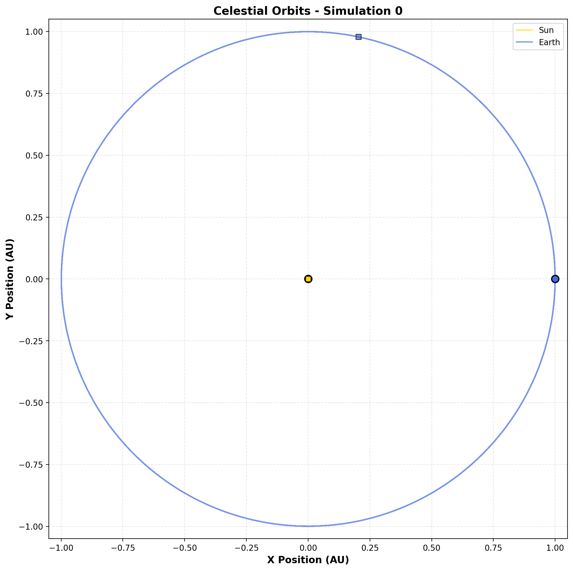
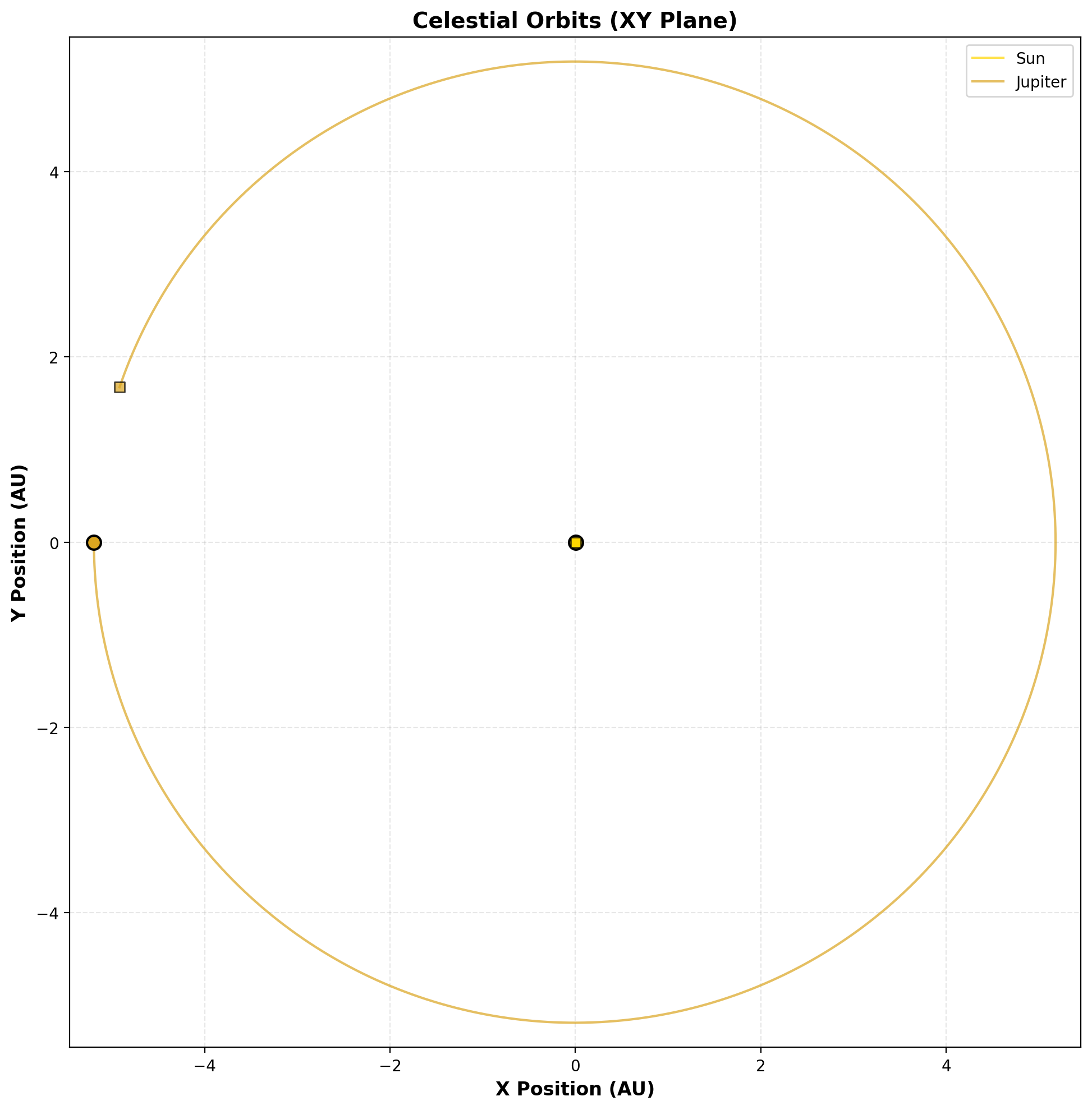
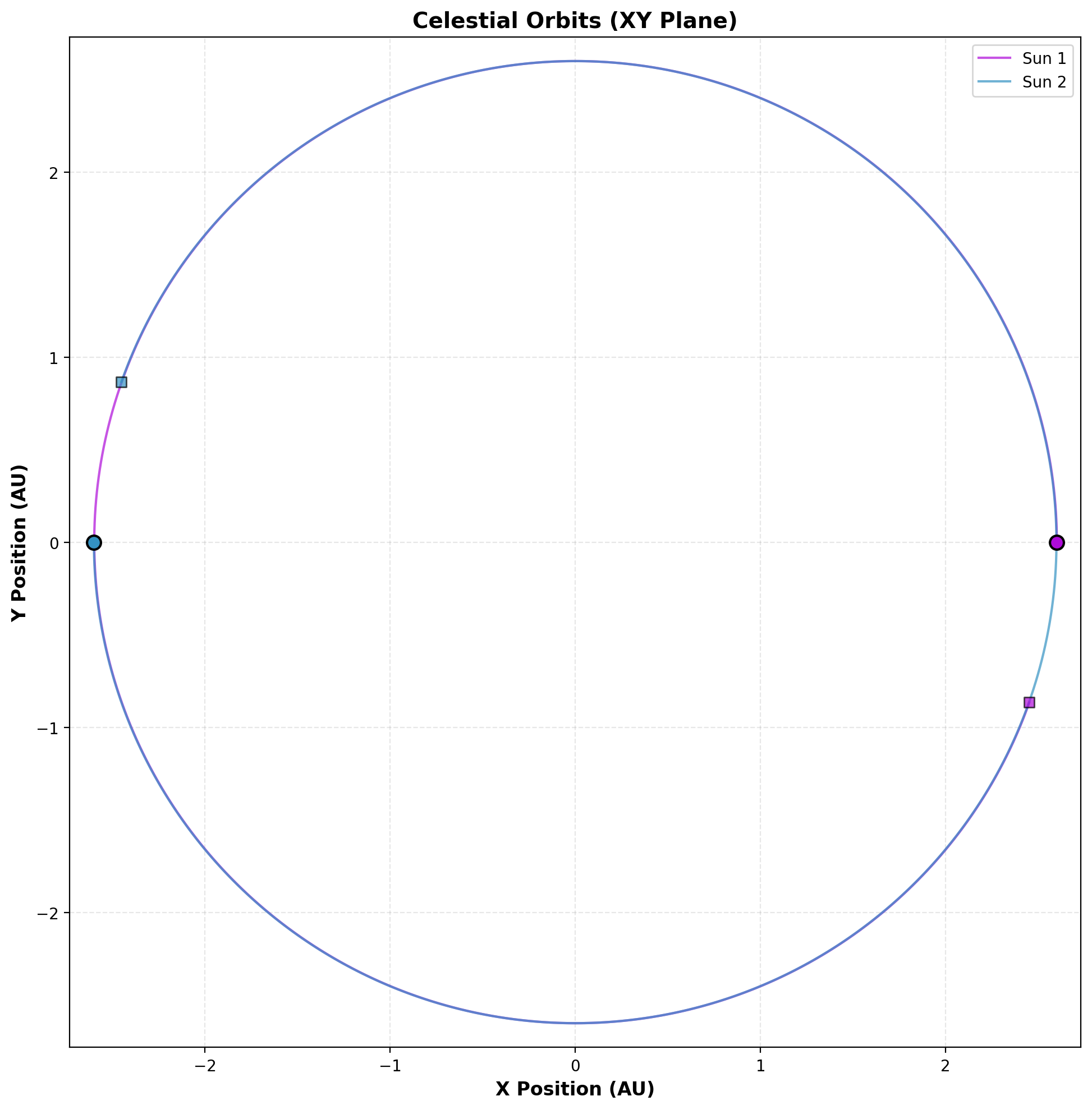
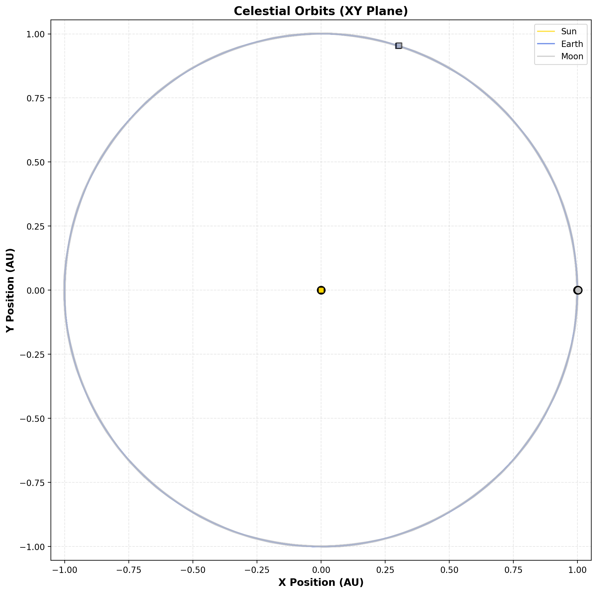
Two-body Earth-Sun orbit Two-body Jupiter-Sun orbit

Three-body Sun-Earth-Moon Three-body with massive Jupiter

2D projections of N-body orbits. Top: two-body Keplerian orbits (Earth-Sun, Jupiter-Sun). Bottom: three-body interactions revealing gravitational perturbations.

3D Orbit Plots

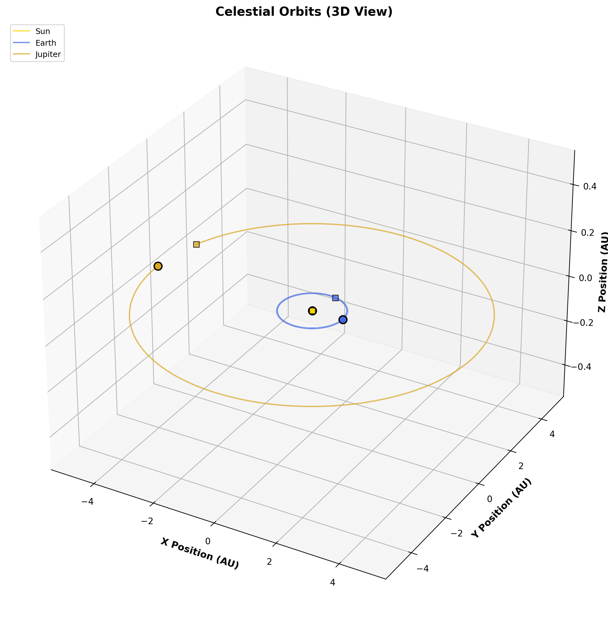
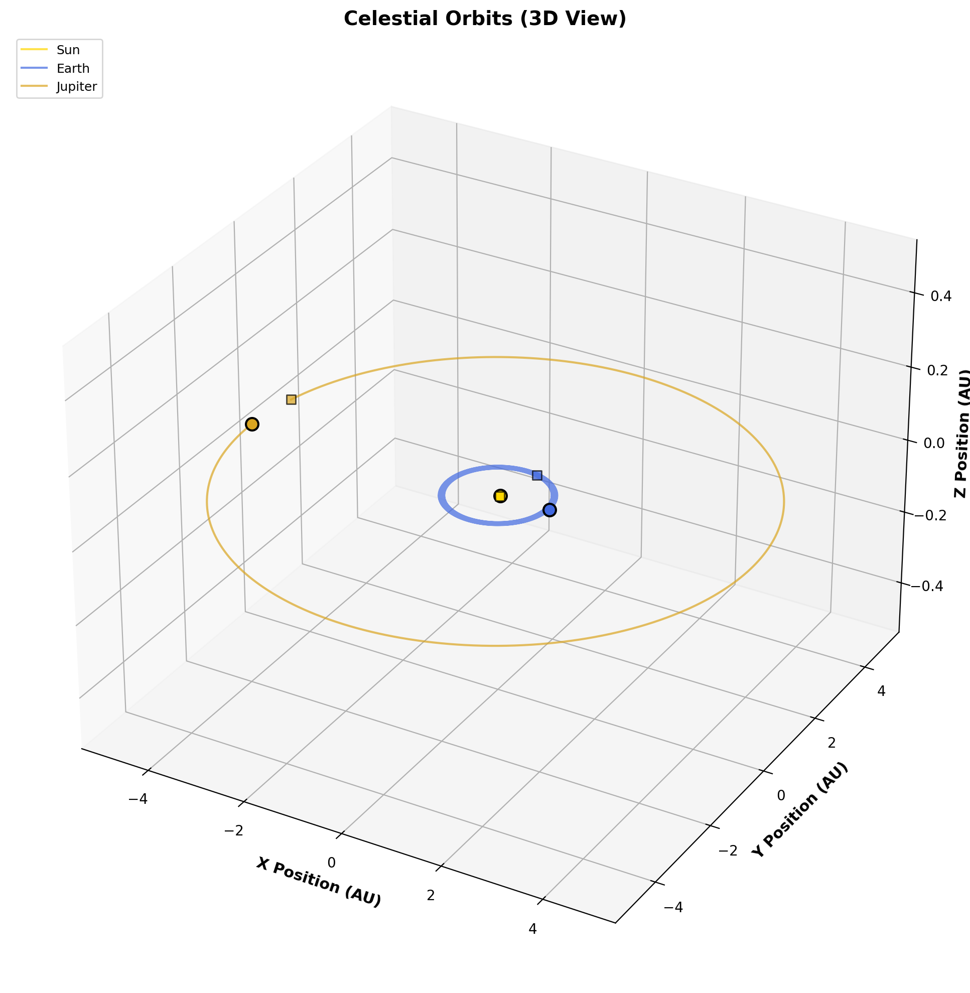
3D orbit visualization 3D solar system subset

3D orbit — orbital inclinations visible 3D orbit — outer planets

3D orbit visualizations showing orbital inclinations and the true spatial structure of planetary systems.

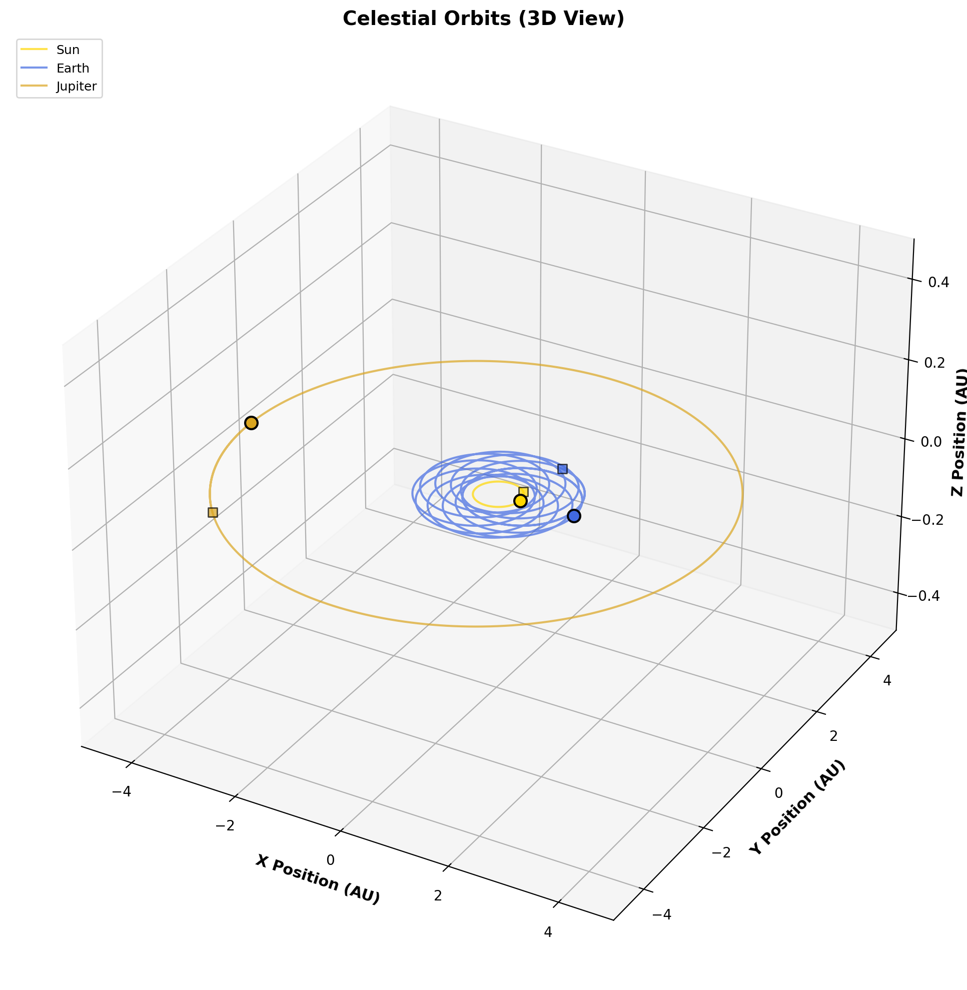
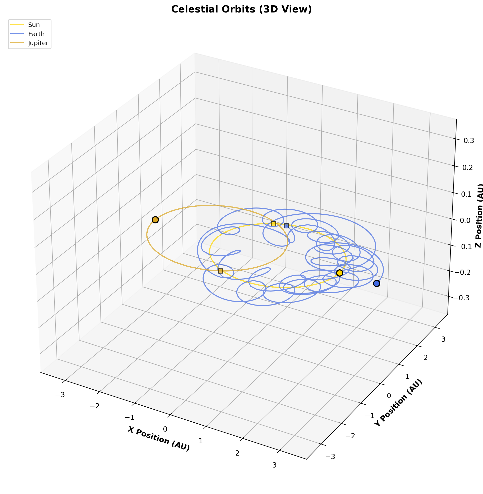
Orbit Animation

3D orbit animation of an N-body gravitational simulation. Planets trace their trajectories over time, illustrating the long-term stability of orbital mechanics under the chosen integrator.

Sources of Error

Source	Nature	Mitigation
Integrator truncation	RK4: $\mathcal{O}(h^4)$; Verlet: $\mathcal{O}(h^2)$; Euler-Cromer: $\mathcal{O}(h)$	Choose integrator based on duration; use smaller $h$ for close encounters
Energy drift (RK4)	Non-symplectic RK4 accumulates secular energy error	Use Verlet or Euler-Cromer for long runs; RK4 for short high-accuracy integrations
Close encounters	Gravitational singularity as $r \to 0$ produces huge accelerations	Softening parameter at $r < 10^{-10}$ AU returns zero force; adaptive time stepping would be better
Two-body approximation	Hardcoded initial conditions assume Keplerian elements at one epoch	Full N-body evolution from accurate initial data; not suitable for billion-year integrations without regularization
No relativistic corrections	GR perihelion precession of Mercury is ~43 arcsec/century	Newtonian gravity only; sufficient for most planetary-scale problems

Computational complexity: $\mathcal{O}(N_\text{bodies}^2 \times N_\text{steps})$ per integration — the gravitational force computation is the dominant cost.

Build & Run

Prerequisites

C++17 compatible compiler (clang++ or g++)
Python 3 with numpy and matplotlib (+ ffmpeg for animations)

Build

make

Run

./bin/main

Follow the interactive prompts to choose simulation type, integrator, time step, and duration. Results are saved to Output/celestial_output_N.csv with auto-incrementing filenames.

Visualize

# Plot a specific simulation
python3 plotting.py 0

# Plot all output files
python3 plotting.py --all

# Plot a specific CSV file
python3 plotting.py path/to/file.csv

Produces Output/celestial_analysis_N_2d.png, Output/celestial_analysis_N_3d.png, and optionally animated .mp4 files.

Simulation Parameters

Configured interactively at runtime:

Parameter	Description	Units
Time step	Integration step $h$	years
Total time	Duration of simulation	years
Integrator	RK4 (1), Euler-Cromer (2), or Verlet (3)	—
Bodies	Any number of `CelestialObject` instances	—

Recommended Settings

Simulation	Time Step	Duration	Integrator
Earth-Sun (1 orbit)	0.0001 yr	1 yr	RK4
Inner Solar System	0.001 yr	10 yr	Verlet
Full Solar System	0.001 yr	200 yr	Verlet
Stability tests (10⁴× Jupiter)	0.0001 yr	50 yr	Verlet

Key Techniques

Technique	Purpose
Three independent integrators (RK4, Euler-Cromer, Verlet)	Compare accuracy vs. energy conservation trade-offs
Backward RK4 bootstrap for Verlet	High-accuracy initialization of $\vec{r}_{-1}$ without Taylor expansion
Automatic center-of-mass centering	Inertial frame; prevents system drift
Template-based integrator design	Generic over state type; reusable across projects
Interactive simulation builder	Explore parameter space without recompiling
729-line Python visualization	2D/3D static plots + animated orbit videos with trail effects
Adjustable Jupiter mass	Probe Solar System stability under gravitational perturbations

Project Structure

Project 3: Celestial Dynamics/
|-- main.cpp                 # Entry point
|-- include/
|   |-- objects.h            # CelestialObject, CelestialSystem, force computation
|   |-- processing.h         # RK4, Euler-Cromer, Verlet integrators (templates)
|   `-- run.h                # Interactive Run class, Solar System data
|-- plotting.py              # 2D/3D orbit plots + animated videos
|-- Makefile                 # Build configuration
|-- bin/                     # Compiled executable
`-- Output/                  # CSV trajectories and PNG/MP4 visualizations
    |-- celestial_output_N.csv
    |-- celestial_analysis_N_2d.png
    `-- celestial_analysis_N_3d.png

Nels Buhrley — Computational Physics, 2025

← Back to Portfolio Hub

Computational Physics & HPC Portfolio

A collection of C++17 numerical simulations spanning classical mechanics, electrostatics, statistical mechanics, molecular dynamics, and number theory — built with OpenMP parallelism and deployed on the BYU Supercomputer.