Project 4: Overrelaxation — 3D Electrostatic Potential Solver
Tip. Every highlighted link in this page is clickable. For fast navagation use Table of Contents
Author: Nels Buhrley
Language: C++17 with OpenMP · Python 3 (visualization)
HPC: Run on the BYU Supercomputer
Build: make release — see Build & Run
Snapshot
- Developed a 3D electrostatic potential solver for Laplace equations using red-black Successive Over-Relaxation in C++17/OpenMP.
- Tuned relaxation strategy and parallel update ordering to accelerate convergence on large grids (up to billion-scale unknown counts).
- Supported realistic Dirichlet configurations (fixed-potential surfaces and embedded charge features) with quantitative convergence tracking.
- Demonstrates strong PDE numerics, parallel iterative solver design, and scalable scientific computing.
For a fast technical check, jump to Algorithm & Parallelism and Results.
Table of Contents
- Snapshot
- Overview
- Physics Background
- Algorithm & Parallelism
- Results
- Sources of Error
- Build & Run
- Simulation Parameters
- Key Techniques
- Project Structure
Overview
This project solves Laplace’s equation $\nabla^2 V = 0$ on a three-dimensional grid using Red-Black Successive Over-Relaxation (SOR) — an iterative relaxation method that converges significantly faster than standard Gauss-Seidel iteration. The solver handles arbitrary Dirichlet boundary conditions including conducting surfaces held at fixed potentials and point charges embedded in the domain. The entire SOR kernel is parallelized with OpenMP, achieving efficient multi-core scaling on grids up to $1000^3$ ($10^9$) unknowns.
Physics Background
Laplace’s Equation
In a charge-free region of space, the electrostatic potential $V(\vec{r})$ satisfies Laplace’s equation:
\[\nabla^2 V = \frac{\partial^2 V}{\partial x^2} + \frac{\partial^2 V}{\partial y^2} + \frac{\partial^2 V}{\partial z^2} = 0\]This is one of the fundamental PDEs in physics, governing not only electrostatics but also steady-state heat conduction, incompressible fluid flow, and gravitational fields in vacuum. Given boundary conditions (voltages on conducting surfaces, charge distributions), the solution $V(\vec{r})$ is unique (Dirichlet’s theorem).
Finite Difference Discretization
The continuous domain is replaced by a uniform cubic grid of $N^3$ points with spacing $\Delta x = L/N$. The Laplacian is approximated by the second-order central difference stencil:
\[\nabla^2 V \approx \frac{V_{i+1,j,k} + V_{i-1,j,k} + V_{i,j+1,k} + V_{i,j-1,k} + V_{i,j,k+1} + V_{i,j,k-1} - 6V_{i,j,k}}{\Delta x^2} = 0\]Solving for $V_{i,j,k}$:
\[V_{i,j,k}^\text{relax} = \frac{1}{6}\left(V_{i+1,j,k} + V_{i-1,j,k} + V_{i,j+1,k} + V_{i,j-1,k} + V_{i,j,k+1} + V_{i,j,k-1}\right)\]Each interior point relaxes toward the average of its six nearest neighbors.
Successive Over-Relaxation (SOR)
Plain Gauss-Seidel iteration ($V_{i,j,k} \leftarrow V^\text{relax}$) converges slowly — $\mathcal{O}(N^2)$ iterations for an $N$-point grid. Over-relaxation accelerates convergence by overshooting toward the relaxed value:
\[V_{i,j,k}^{(n+1)} = (1 - \omega)\,V_{i,j,k}^{(n)} + \omega\,V_{i,j,k}^\text{relax}\]where the relaxation parameter $\omega \in (1, 2)$ controls the overshoot. The optimal value for a cubic grid is:
\[\omega_\text{opt} = \frac{2}{1 + \sin(\pi/N)}\]which reduces the iteration count from $\mathcal{O}(N^2)$ to $\mathcal{O}(N)$ — a dramatic speedup for large grids. This optimal $\omega$ is computed automatically in the constructor.
Red-Black Ordering
Standard SOR has a sequential dependency: updating point $(i,j,k)$ reads neighbors that may have already been updated in the same sweep. Red-black (checkerboard) ordering eliminates this dependency by partitioning the grid into two disjoint sets:
- Red points: $(i + j + k)$ even
- Black points: $(i + j + k)$ odd
All red points depend only on black neighbors and vice versa. Within each color, all updates are independent and can be executed in any order — or in parallel. A full iteration consists of one red sweep followed by one black sweep.
Test Configuration
The default boundary conditions configure:
- A conducting disk of ~10 cm radius centered in the domain, held at $V = 0.25$ V
- Point charges of $\pm 1\;\mu\text{C}$ at positions offset by 25 cm along the $x$ and $y$ axes from center
The point-charge voltage is computed from Coulomb’s law:
\[V = \frac{q}{4\pi\varepsilon_0 r}\]and applied as a Dirichlet constraint over a small sphere ($r = 1$ cm) surrounding each charge location.
Algorithm & Parallelism
OpenMP Parallelization
The SOR kernel is the computational bottleneck, performing $\mathcal{O}(N^3)$ floating-point operations per iteration across up to $8N$ iterations. Four regions are parallelized:
| Region | Directive | Scheduling | Purpose |
|---|---|---|---|
redOrBlackUpdate() |
#pragma omp parallel for collapse(2) schedule(static) |
Static | Core SOR kernel — updates all points of one color in parallel |
computeResidual() |
#pragma omp parallel for reduction(+:residual_squared) collapse(3) schedule(static) |
Static + reduction | $L^2$ residual norm with thread-safe accumulation |
| Grid initialization | #pragma omp parallel for collapse(3) schedule(static) |
Static | Zero-fill $u$ and $f$ arrays |
| CSV output | #pragma omp parallel for schedule(static) |
Static | Parallel string formatting partitioned by thread |
The collapse(2) on the SOR kernel merges the outer two loops ($i$ and $j$) into a single parallel iteration space, exposing $\mathcal{O}(N^2)$ independent chunks to OpenMP. The inner $k$-loop is sequential within each chunk but strides by 2 to visit only the target color, maintaining the red-black invariant.
Convergence Monitoring
The $L^2$ residual norm is computed every 100 iterations:
\[R = \sqrt{\sum_{i,j,k} \left(\nabla^2_h V_{i,j,k}\right)^2}\]where $\nabla^2_h$ is the discrete Laplacian. The simulation converges when $R < \varepsilon$ (default $\varepsilon = 4 \times 10^{-10}$) or after $8N$ maximum iterations.
Results
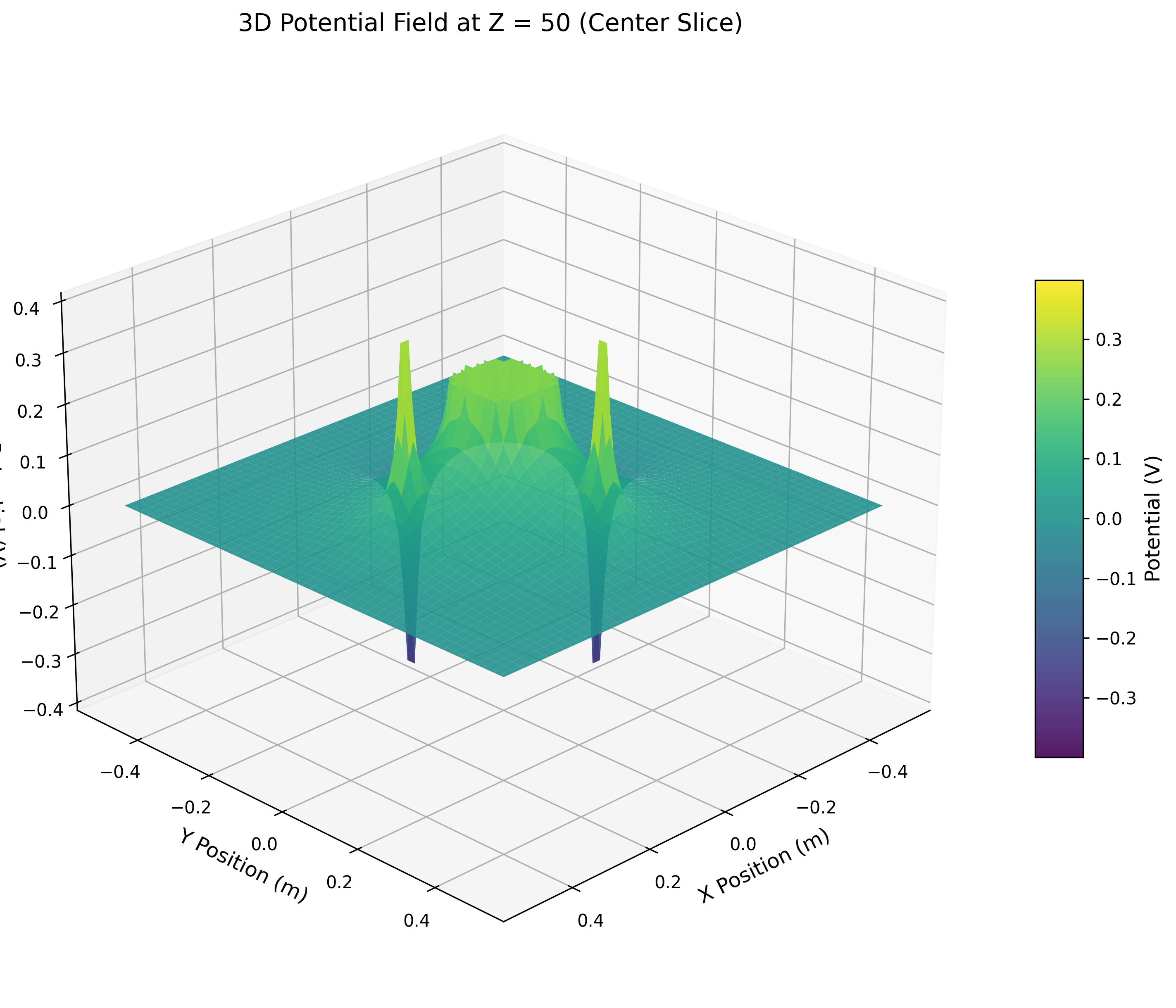
2D slice through the 3D electrostatic potential field at different $z$-planes. The conducting disk (center) and dipole point charges (offset) create the characteristic equipotential structure. Color maps the potential magnitude.
Interactive 3D Visualization
The interactive plot above renders the same 3D electrostatic potential field as the static slice, but with full rotational control and a z-axis slider. You can:
- Rotate the 3D volume by dragging your mouse to inspect the potential structure from any angle
- Zoom using the scroll wheel to examine fine details
- Slide through z-planes with the slider to reveal how the field evolves along the depth axis in real time
This allows intuitive exploration of the dipole and disk geometry without generating dozens of static images.
Sources of Error
| Source | Nature | Mitigation |
|---|---|---|
| Spatial discretization | Second-order central differences: error $\mathcal{O}(\Delta x^2)$ | Increase $N$; error quarters when grid doubles |
| Convergence tolerance | Residual $R > 0$ means the solution is approximate | Tighten tolerance; default $4 \times 10^{-10}$ is stringent |
| Point-charge singularity | $V \to \infty$ at exact charge location; discretized over a small sphere | Sphere radius = 1 cm; finer grids resolve the near-field better |
| Boundary effects | Domain walls at $V = 0$ (grounded); close walls distort the field | Use large domain relative to charge separation; $N = 1000$ with 1 m cube gives 1 mm resolution |
| Floating-point accumulation | $10^9$ additions per iteration; round-off accumulates | double precision; residual monitored explicitly |
Computational complexity:
- Per iteration: $\mathcal{O}(N^3)$
- Total: $\mathcal{O}(N^4)$ with optimal $\omega$ (vs. $\mathcal{O}(N^5)$ for Gauss-Seidel)
- Default parameters ($N = 1000$): ~5 minutes wall time on an 8-thread machine
Build & Run
Prerequisites
- C++17 compatible compiler (
clang++org++) - OpenMP (
brew install libompon macOS) - zlib (for
.npzoutput viacnpy) - Python 3 with
numpyandmatplotlib(for visualization)
Build
make release    # Optimized build (-O3, march=native, OpenMP)
make debug      # Debug build (no optimization)
make clean      # Remove build artifacts
Run
./bin/main
Output is saved to output.csv and output.npz.
Output Format
| File | Contents |
|---|---|
output.csv |
Hierarchical text: nested by $z$, $y$, $x$ layers with potential values |
output.npz |
NumPy array potential of shape $(N, N, N)$ — load with np.load("output.npz")["potential"] |
Simulation Parameters
Configured in main.cpp:
| Parameter | Default | Description |
|---|---|---|
N |
1000 | Cubic grid edge length ($N^3$ unknowns) |
physicalDimensions |
1.0 m | Physical size of the simulation cube |
tolerance |
4×10⁻¹⁰ | Convergence threshold on $L^2$ residual |
| $\omega$ \lvertauto\rvert Optimal SOR parameter $2/(1 + \sin(\pi/N))$ | ||
| Max iterations | $8N$ | Safety limit |
Key Techniques
| Technique | Purpose |
|---|---|
| Red-Black Successive Over-Relaxation | $\mathcal{O}(N)$ convergence vs. $\mathcal{O}(N^2)$ for Gauss-Seidel |
| Optimal $\omega = 2/(1 + \sin(\pi/N))$ | Minimizes iteration count analytically |
| Red-black checkerboard decomposition | Eliminates update dependencies; enables safe parallelism |
collapse(2) OpenMP kernel |
Exposes $N^2$ independent work units to thread pool |
reduction(+:residual_squared) |
Thread-safe residual accumulation without locks |
Dirichlet boundary via source array f[] |
Boundary points held fixed; interior points relaxed freely |
| Point-charge voltage from Coulomb’s law | Physically correct embedded charge boundary conditions |
NPZ output via cnpy |
Compressed, self-describing format for direct NumPy loading |
Project Structure
Project 4: Overrelaxation/
|-- main.cpp        # Entry point: configures grid, charges, runs SOR
|-- Processing.h    # PotentialField class: SOR kernel, residual, I/O
|-- Makefile        # Build targets: release, debug, profile-guided
|-- bin/            # Compiled executable
|-- output.csv      # Full 3D potential (hierarchical text)
|-- output.npz      # Full 3D potential (NumPy compressed)
`-- output/         # Visualization outputs (PNG slices)
Nels Buhrley — Computational Physics, 2025