Project 5: Oscillations on a String
Tip. Every highlighted link in this page is clickable. For fast navagation use Table of Contents
Author: Nels Buhrley
Language: C++17 with OpenMP · KissFFT · Python 3 (visualization)
Build: make release — see Build & Run
Snapshot
- Built a finite-difference wave solver for damped, stiff-string dynamics with configurable initial-condition composition.
- Integrated spectral diagnostics using KissFFT to extract mode content and mean power spectra from spatiotemporal simulation output.
- Parallelized core updates with OpenMP and shipped compressed output workflows for efficient post-processing.
- Demonstrates combined strengths in PDE simulation, frequency-domain analysis, and performance-oriented implementation.
For a fast technical check, jump to Algorithmic Design and Visualization.
Table of Contents
- Snapshot
- Overview
- Physics Background
- Algorithmic Design
- Parallelization Strategy
- Sources of Error and Limitations
- Visualization
- Results
- Build & Run
- Simulation Parameters
- Key Techniques at a Glance
- Project Structure
Overview
This project implements a finite difference simulation of transverse wave propagation on a damped, stiff string, with full spectral analysis of the resulting oscillations via the Fast Fourier Transform. The simulation captures the rich physics of wave superposition, dispersion due to bending stiffness, and energy dissipation through damping — all of which arise in real-world string instruments, structural cables, and fiber-optic waveguides.
Initial conditions are built by superimposing any number of Gaussian pulse disturbances, sine waves, or natural harmonic modes directly onto the string. The simulation then evolves the full spatiotemporal displacement field $u(x, t)$, computes the per-point and mean power spectrum across all positions, and saves everything to compressed .npz archives for visualization.
Physics Background
The Wave Equation
The idealized transverse displacement $u(x, t)$ of a flexible string under tension $T$ and linear mass density $\mu$ satisfies the classical wave equation:
\[\frac{\partial^2 u}{\partial t^2} = c^2 \frac{\partial^2 u}{\partial x^2}\]where the wave speed is $c = \sqrt{T/\mu}$. This admits travelling wave solutions of the form $u = f(x \pm ct)$ and, for a string of length $L$ with fixed ends, a discrete set of normal modes (standing waves) at frequencies:
\[f_n = \frac{n c}{2L}, \qquad n = 1, 2, 3, \ldots\]The lowest frequency $f_1 = c / 2L$ is the fundamental, and the higher modes $f_n = n f_1$ are harmonics. This harmonic series is the physical origin of musical pitch in stringed instruments.
Bending Stiffness
A real string or beam resists bending. Adding a bending rigidity term $EI$ (flexural stiffness) modifies the wave equation to the Euler–Bernoulli beam equation:
\[\frac{\partial^2 u}{\partial t^2} = c^2 \frac{\partial^2 u}{\partial x^2} - \kappa^2 \frac{\partial^4 u}{\partial x^4}\]where $\kappa^2 = EI/\mu$ is the stiffness coefficient. The fourth-order spatial derivative introduces dispersion: higher-frequency modes travel at different speeds, causing wavepackets to spread over time. This is captured in the simulation through the stiffness parameter and the corresponding update stencil that reaches two grid points to either side.
Damping
Physical strings dissipate energy through internal friction and air resistance. A linear damping term proportional to velocity $\partial u / \partial t$ extends the equation to:
\[\frac{\partial^2 u}{\partial t^2} = c^2 \frac{\partial^2 u}{\partial x^2} - \kappa^2 \frac{\partial^4 u}{\partial x^4} - \gamma \frac{\partial u}{\partial t}\]where $\gamma$ is the damping coefficient. This causes all modes to decay exponentially in time, with higher modes decaying faster — consistent with the observed behavior of plucked strings.
Power Spectrum and Normal Modes
After the simulation runs, the time series $u(x_i, t)$ at each spatial point $x_i$ is transformed into the frequency domain via the Discrete Fourier Transform. The power $P(f) \propto \lvert\hat{u}(f)\rvert^2$ reveals which frequencies are excited and how strongly. Averaging over all spatial positions gives the mean power spectrum, which clearly shows peaks at the normal mode frequencies $f_n$ — a direct verification of the wave physics.
Algorithmic Design
Finite Difference Discretization
The continuous string is replaced by a uniform grid of $N$ spatial points separated by $\Delta x = L / N$ (stepSize) and advanced in time steps of $\Delta t$ (timeStep). The second- and fourth-order spatial derivatives are approximated by standard central differences:
Substituting into the damped stiff wave equation with the explicit time-stepping scheme and introducing the Courant number $r = c \Delta t / \Delta x$ yields the full update formula, implemented exactly in simulate():
where superscripts are time indices and subscripts are spatial indices. The division by $(1 + \gamma \Delta t)$ implements the implicit damping correction that keeps the scheme stable under dissipation.
Courant–Friedrichs–Lewy (CFL) Stability Condition
Explicit finite-difference schemes for the wave equation are only conditionally stable: if $\Delta t$ is too large relative to $\Delta x$, numerical errors grow exponentially and the simulation diverges. The stability condition for the pure wave equation is $r \leq 1$. With added stiffness the condition tightens to:
\[r \leq \frac{1}{\sqrt{1 + 4\kappa N^2}}\]Rather than requiring the user to compute this, the constructor automatically computes $r$ and derives $\Delta t$ from it:
r = 0.95 / std::sqrt(1.0 + 4.0 * stiffness * segments * segments);
timeStep = r * length / segments / waveSpeed;
The factor of $0.95$ provides a $5\%$ safety margin below the theoretical stability limit. This design means the simulation is unconditionally stable by construction regardless of the stiffness or grid resolution chosen — the time step adapts automatically.
Initial Conditions: Superposition API
Initial conditions are set by superimposing contributions onto the $t=0$ displacement row using a clean, composable API:
| Method | Physics |
|---|---|
superemposeGaussian(center, width, amplitude) |
Localized pulse — mimics a pluck or strike |
superemposeSine(frequency, amplitude) |
Pure-frequency excitation |
superemposeNaturalMode(n, amplitude) |
Exact $n$-th standing-wave eigenmode |
Multiple calls accumulate additively, so any superposition of initial conditions is possible. Each method is parallelized internally with #pragma omp parallel for.
Boundary Conditions
The simulation supports fixed ends (endIsFixed = true), enforcing $u(0, t) = u(L, t) = 0$. At the boundaries, the stencil requires values outside the domain ($i-2$ or $i+2$). These are obtained by odd reflection (mirror with sign flip), which is the correct ghost-cell boundary condition for a fixed end:
secondSpaceTermPlus  = (i < segments - 2) ? u[t-1][i+2] : -u[t-1][i+1];
secondSpaceTermMinus = (i > 1)            ? u[t-1][i-2] : -u[t-1][i-1];
This antisymmetric extension ensures the displacement is exactly zero at the wall, with no spurious reflections from the truncation.
Spectral Analysis with KissFFT
After simulation, FFTallPoints() computes the Discrete Fourier Transform of the time series at every spatial point using KissFFT — a lightweight, dependency-free FFT library included directly in the project (no external install required).
Two optimizations are applied:
-
Zero-padding to next fast size:
kiss_fft_next_fast_size(timeSteps)finds the smallest integer $\geq N_t$ whose prime factorization contains only small primes (2, 3, 5), ensuring the FFT runs at maximum speed. The signal is zero-padded to this length before transformation. -
One-sided spectrum: Since the input is real-valued, the FFT output is Hermitian-symmetric. Only the first $N/2 + 1$ bins are unique and are retained, halving the storage and computation needed for the power spectrum.
The mean power spectrum is then computed as the spatial average of $\lvert\hat{u}(f)\rvert^2$ across all points — a single serial pass over bins and segments, avoided from parallelization to prevent accumulation race conditions.
Parallelization Strategy
| Region | OpenMP pattern | Scheduling | Rationale |
|---|---|---|---|
Initial condition setup (superempose*) |
#pragma omp parallel for |
static |
Spatial points are independent; equal work per point |
simulate() spatial loop |
#pragma omp parallel for (inside sequential time loop) |
static |
Particle loop is independent; time loop must stay sequential |
FFTallPoints() |
#pragma omp parallel for (after serial init) |
static |
Each spatial point’s FFT is completely independent |
outputPositionResultsCSV() row building |
#pragma omp parallel for |
static |
Each row is an independent string; written serially after |
Why the Time Loop Stays Sequential
The update formula at step $t$ reads from steps $t-1$ and $t-2$. This is an irreducible sequential dependency: no thread can compute step $t$ until all spatial points at $t-1$ are finished. OpenMP’s implicit barrier at the end of each #pragma omp for enforces this automatically — all threads complete the spatial sweep before any begins the next time step.
--- Sequential ---------------------------------------------------------------
for t = 1 ... timeSteps:
    --- Parallel -------------------------------------------------------------
    #pragma omp parallel for
    for i = 1 ... N-1:   u[t][i] = f(u[t-1], u[t-2])
    --- [implicit barrier: all threads sync before t+1] ----------------------
FFT Race Condition Prevention
fftFrequencies (the frequency axis) is shared across threads but must only be written once. To prevent a race where multiple threads simultaneously initialize it, one serial FFT is run before the parallel region to populate fftFrequencies and size fftMagnitudes. The parallel loop then finds both already initialized and writes only to its own private row — no locks needed:
if (fftFrequencies.empty()) FFTatPoint(0);   // Serial init: populates shared state
if (fftMagnitudes.size() != segments) ...    // Resize once before parallel region
#pragma omp parallel for schedule(static)
for (int i = 0; i < segments; i++) FFTatPoint(i);  // Each i writes only fftMagnitudes[i]
Sources of Error and Limitations
| Source | Nature | Mitigation |
|---|---|---|
| Spatial truncation error | Central difference is $\mathcal{O}(\Delta x^2)$ accurate | Increase segments; error quarters with each doubling of grid |
| Temporal truncation error | Explicit scheme is $\mathcal{O}(\Delta t^2)$ accurate | $\Delta t$ is auto-chosen at 95% of the stability limit |
| Numerical dispersion | Finite difference stencils introduce a speed error that grows with frequency | Use finer grids; higher-order stencils |
| CFL instability | If stiffness or grid is changed manually outside the constructor | Always construct via the string(...) Class — $r$ is computed automatically |
| Spectral leakage | FFT assumes periodicity; non-periodic signals leak power between bins | Apply a windowing function (e.g., Hann) to the time series before FFT |
| Fixed boundary only | Free-end boundary conditions noted as not yet implemented | Extend the ghost-cell logic in simulate() for Neumann conditions |
Computational complexity:
\[\mathcal{O}(N_t \times N_x) \quad \text{(simulation)} \;+\; \mathcal{O}(N_x \times N_t \log N_t) \quad \text{(FFT)}\]The FFT step dominates for long simulations, but is fully parallelized across spatial points.
Visualization
The Python script plotting.py loads the .npz archive and produces a single composite figure with three panels, plus a saved MP4 animation.
Figure Layout
+------------------------+------------------------+
|  Initial Displacement  |   Mean Power Spectrum  |
|       (t = 0)          |     (log-scale, Hz)    |
+------------------------+------------------------+
|         String Propagation Animation            |
|           (full time evolution)                 |
+-------------------------------------------------+
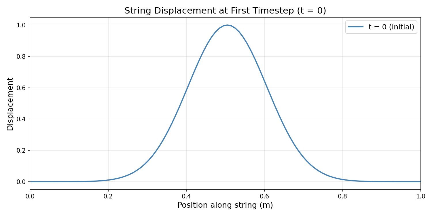
Panel 1 — Initial String Displacement: A static line plot of $u(x, 0)$, showing the superimposed Gaussian pulses as the starting condition.
Panel 2 — Mean Power Spectrum: A semi-log plot of the spatially averaged power $\langle \lvert\hat{u}(f)\rvert^2 \rangle_x$ vs frequency. Peaks correspond to the excited normal modes of the string. The frequency axis is automatically clipped to the range containing significant power, keeping the plot readable regardless of simulation length.
Panel 3 — Animation: A live line plot of the string profile $u(x, t)$ stepped through time, saved to string_oscillations.mp4 via ffmpeg. The title updates to show the simulated time in seconds.
Animation controls (top of plotting.py):
| Parameter | Default | Effect |
|---|---|---|
fps |
5 | Playback frame rate of the saved MP4 |
duration_s |
180 | Target animation length in seconds |
max_time_index |
100 000 | Caps the data range animated (for very long runs) |
Data Format
| Array in NPZ | Shape | Description |
|---|---|---|
positions |
(timeSteps, segments) |
Full spatiotemporal displacement field $u(x, t)$ |
frequencies |
(numBins,) |
Frequency axis in Hz |
fft_magnitudes |
(segments, numBins) |
FFT magnitude at every spatial point |
mean_power_spectrum |
(numBins,) |
Spatially averaged power per frequency bin |
parameters |
(5,) |
[length, waveSpeed, stiffness, r, timeStep] |
Loading in Python:
import numpy as np
data = np.load("string_oscillations.npz")
u    = data["positions"]           # shape: (timeSteps, segments)
freq = data["frequencies"]         # shape: (numBins,)
pwr  = data["mean_power_spectrum"] # shape: (numBins,)
L, c, kappa, r, dt = data["parameters"]
Results
Initial String Displacement
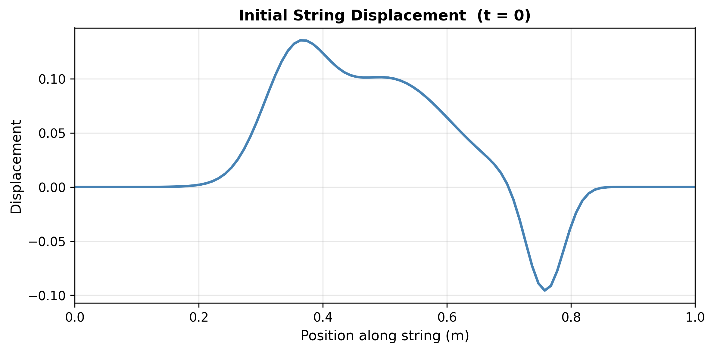
Initial displacement profile $u(x, 0)$ showing three superimposed Gaussian pulses at different positions, widths, and amplitudes. This is the starting condition before time evolution.
Mean Power Spectrum
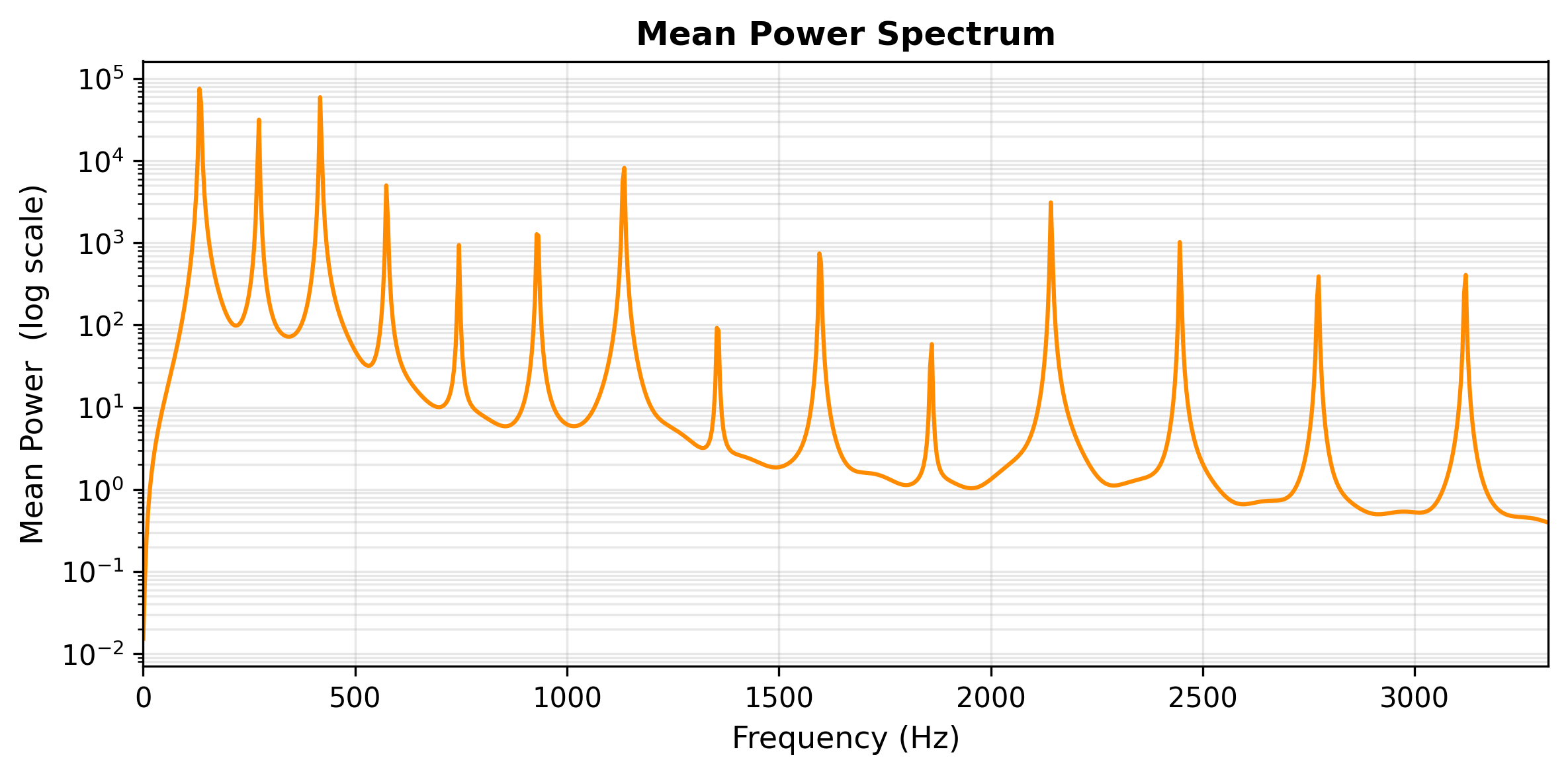
Spatially averaged power spectrum $\langle \lvert\hat{u}(f)\rvert^2 \rangle_x$ revealing the excited normal-mode frequencies. Peaks at $f_n = nc/2L$ confirm the standing-wave structure predicted by the wave equation.
String Propagation
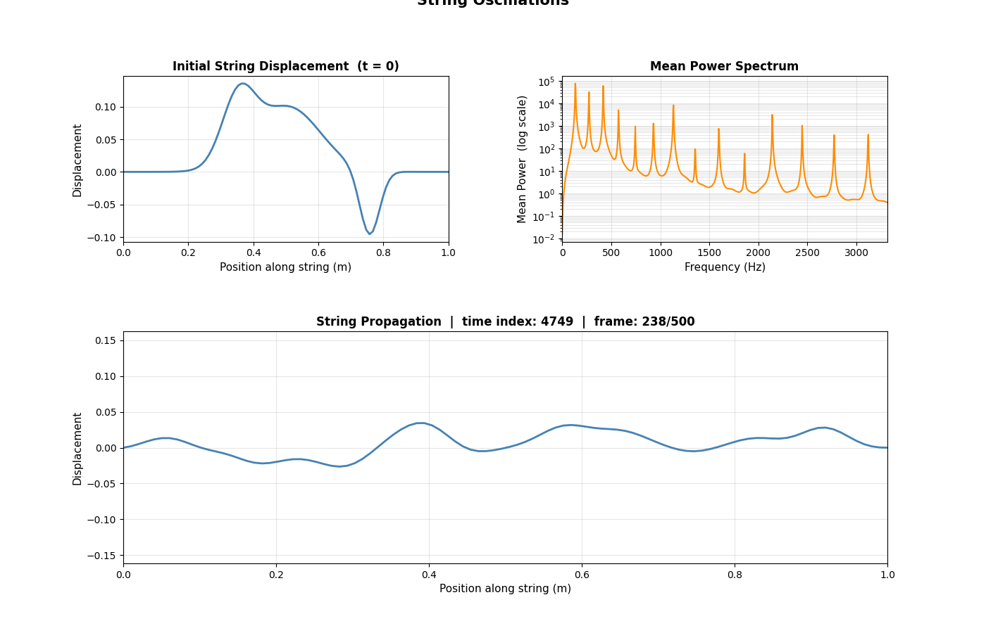
Left: snapshot of the string displacement during time evolution. Right: initial state reference. The interplay of reflection, superposition, and damping shapes the evolving waveform.
String Oscillation Animation
Animation of the transverse displacement $u(x, t)$ evolving over the full simulation. The three superimposed Gaussian pulses propagate, reflect off the fixed ends, and gradually lose amplitude due to damping, illustrating the interplay of wave superposition and energy dissipation on a stiff string.
Build & Run
Prerequisites
- C++17 compatible compiler (
clang++org++) - OpenMP (via Homebrew:
brew install libompon macOS) - zlib (for
.npzcompression) - KissFFT — included in the project directory (no install required)
- Python 3 with
numpy,matplotlib, andffmpeg(for visualization and animation export)
Build
# Optimized release build (recommended)
make release

# Debug build (full warnings, no optimization)
make debug

# Profile-guided optimization (two-step)
make profile-gen && ./bin/main && make profile-use
Run
./bin/main
Output is written to string_oscillations.npz (and matching .csv files) in the current directory.
Visualize
python3 plotting.py
Simulation Parameters
Configured in main.cpp:
| Parameter | Default | Description |
|---|---|---|
length |
1.0 m | Physical length of the string |
waveSpeed |
250.0 m/s | Transverse wave speed $c = \sqrt{T/\mu}$ |
segments |
100 | Number of spatial grid points |
stiffness |
0.001 | Bending stiffness coefficient $\kappa$ |
damping |
10 | Linear damping coefficient $\gamma$ |
endIsFixed |
true |
Fixed-end boundary conditions |
totalTime |
0.25 s | Duration of the simulation |
Note:
randtimeStepare derived automatically from these parameters to guarantee CFL stability. Do not set them manually.
Default Initial Condition
Three Gaussian pulses are superimposed at setup:
testString.superemposeGaussian(0.50, 0.10,  0.1);   // centre pulse
testString.superemposeGaussian(0.35, 0.05,  0.1);   // left pulse
testString.superemposeGaussian(0.75, 0.03, -0.1);   // right pulse (inverted)
To excite a specific normal mode instead, comment those lines and use:
testString.superemposeNaturalMode(3, 0.5); // third harmonic
Project Structure
Project 5: Occilations on a string/
|-- main.cpp              # Entry point: configures string, sets ICs, runs simulation
|-- processing.h          # string class: FD solver, FFT, CSV and NPZ output
|-- kiss_fft.h / .c       # KissFFT library (included, no external dependency)
|-- _kiss_fft_guts.h      # KissFFT implementation internals
|-- kiss_fft_log.h        # KissFFT logging utilities
|-- Makefile              # Multi-target build: debug, release, profile-guided
|-- plotting.py           # Python visualization: 3-panel figure + MP4 animation
`-- output/
    |-- string_oscillations.npz             # Full simulation data (NumPy archive)
    |-- string_oscillations_positions.csv   # Spatiotemporal displacement (CSV)
    `-- string_oscillations_spectrum.csv    # Mean power spectrum (CSV)
Key Techniques at a Glance
| Technique | Purpose |
|---|---|
| Finite difference discretization of the stiff wave equation | Numerically stable spatiotemporal evolution without solving differential equations analytically |
| Automatic CFL time-step selection with 5% safety margin | Guarantees stability for any choice of grid resolution and stiffness |
| Fourth-order spatial stencil for bending rigidity | Captures dispersion effects absent from the simple wave equation |
| Odd-reflection ghost cells at fixed boundaries | Enforces zero-displacement BCs branch-free, with no special cases in the inner loop |
| Sequential time loop + parallel spatial loop | Respects the $t \to t+1$ dependency while fully utilizing available CPU cores |
| Serial FFT initialization before parallel region | Prevents race conditions on shared frequency-axis state without any locks |
| KissFFT with zero-padding to next fast size | Maximizes FFT efficiency; avoids slow prime-size transforms |
| One-sided Hermitian spectrum | Halves memory and compute for real-valued input signals |
| Parallel CSV row building with sequential write | Eliminates I/O serialization for large output files |
NPZ archive with self-describing parameters array |
Single-file, compressed, self-contained data portable to any NumPy environment |
Nels Buhrley — Computational Physics, 2026