Project 6: 3D Random-Walk Diffusion Simulation
Tip. Every highlighted link in this page is clickable. For fast navagation use Table of Contents
Author: Nels Buhrley
Language: C++17 with OpenMP · Python 3 (visualization)
HPC: Run on the BYU Supercomputer
Build: make release — see Build & Run
Snapshot
- Implemented a 3D Monte Carlo diffusion simulator that tracks large particle ensembles under reflective boundary constraints.
- Used OpenMP to parallelize independent random-walk trajectories and scale ensemble statistics efficiently on multicore/HPC resources.
- Validated outputs against diffusion theory by measuring RMS displacement and linear mean-squared-displacement trends.
- Demonstrates stochastic simulation design, statistical validation, and high-throughput scientific computation.
For a fast technical check, jump to Algorithmic Design and Results.
Table of Contents
- Snapshot
- Overview
- Physics Background
- Algorithmic Design
- Parallelization Strategy
- Sources of Error and Limitations
- Visualization
- Results
- Build & Run
- Simulation Parameters
- Key Techniques at a Glance
- Project Structure
Overview
This project implements a Monte Carlo simulation of three-dimensional diffusion by tracking an ensemble of independent particles undergoing fixed-step random walks inside a reflective cubic volume.
Imagine dropping a single drop of dye into a still glass of water. Over time the dye spreads outward in every direction, not because of any directed force, but because each molecule is being jostled billions of times per second by the surrounding water molecules. This spreading — Brownian diffusion — emerges from pure randomness at the microscopic scale. This simulation models exactly that process: each particle represents a diffusing molecule, each time step is one random collision event, and the cubic volume is the confining geometry of the container.
The tool is deliberately general. The same algorithm describes diffusion of gas molecules in a box, charge carriers in a disordered semiconductor, bacteria performing a run-and-tumble search, or photons scattering through a turbid medium. The step size and box size can be tuned to match any physical scale of interest.
Physics Background
Brownian Motion and the Random Walk
In 1905 Einstein showed that the macroscopic phenomenon of diffusion arises from the statistical accumulation of microscopic random displacements. For a particle undergoing a 3D random walk with step length $\ell$ and taking $n$ steps per second, the mean squared displacement (MSD) from the starting point grows linearly in time:
\[\langle r^2(t) \rangle = 6 D t\]where $D$ is the diffusion coefficient, related to the step size by:
\[D = \frac{\ell^2}{6 \tau}\]with $\tau$ the mean time between steps. The factor of $6 = 2d$ where $d = 3$ is the spatial dimension. This linear growth — verified experimentally by Perrin in 1908 — is the defining signature of normal diffusion and is what the simulation measures.
Root-Mean-Square Displacement
The observable computed after each step is the RMS displacement:
\[r_\text{RMS}(t) = \sqrt{\langle r^2(t) \rangle} = \sqrt{\frac{1}{N} \sum_{i=1}^{N} \left( x_i^2 + y_i^2 + z_i^2 \right)}\]where the sum is over all $N$ independent particles. Squaring the RMS gives the MSD, whose slope encodes the diffusion coefficient $D$. The simulation outputs both $r_\text{RMS}$ (for inspection) and the squared version plotted against step number so the expected linear trend is directly visible.
Reflective Boundary Conditions
Real diffusion in a container is bounded. When a particle reaches a wall it does not disappear — it reflects. This simulation implements specular (mirror) reflection: if a proposed new coordinate $x’$ would exceed the boundary $\pm L/2$, the overshoot is folded back:
\[x \leftarrow \begin{cases} -L - x' & x' < -L/2 \\ L - x' & x' > +L/2 \end{cases}\]This preserves the particle’s speed and total path length while keeping the particle inside the box, consistent with an elastic collision with a hard wall.
Uniform Sampling on the Unit Sphere
The most subtle physics is ensuring that random step directions are uniformly distributed on the 3D unit sphere. A naive approach of sampling $\theta$ and $\phi$ uniformly in $[0, \pi]$ and $[0, 2\pi)$ and converting to Cartesian coordinates introduces a polar bias — directions crowd near the poles because equal increments of $\theta$ correspond to progressively smaller areas as $\theta \to 0$ or $\pi$. This would cause the simulated diffusion to be anisotropic and unphysical.
The correct method samples the cosine of the polar angle uniformly:
\[\cos\phi \sim \mathcal{U}(-1, +1), \qquad \theta \sim \mathcal{U}(0, 2\pi)\]which is derived from the area element of the sphere $dA = \sin\phi \, d\phi \, d\theta = -d(\cos\phi) \, d\theta$. Using two uniform random numbers $u, v \in [0, 1)$:
\[\theta = 2\pi u, \qquad \cos\phi = 1 - 2v, \qquad \sin\phi = \sqrt{1 - \cos^2\phi}\]The displacement vector is then:
\[\Delta \vec{r} = r \begin{pmatrix} \sin\phi \cos\theta \\ \sin\phi \sin\theta \\ \cos\phi \end{pmatrix}\]where $r$ is the fixed step length movementRadius. This guarantees isotropy — no direction in space is preferred over any other.
Algorithmic Design
Data Structure
All particle positions are stored in a single 3D structure:
points[step][particle] = { x, y, z }
The outermost dimension indexes time (steps), the next indexes particles, and the innermost holds the three spatial coordinates as std::array<float, 3>. This layout means that all particles at a given step are contiguous in memory, which is exactly the access pattern of the parallel inner loop, maximizing cache efficiency during the propagation sweep.
Simulation Loop Structure
The propagation must respect a strict dependency: the position of particle $i$ at step $t$ depends on its position at step $t-1$. This makes the step dimension sequential and the particle dimension embarrassingly parallel:
Sequential:  for each step t = 1 ... N_steps
    Parallel:  for each particle i = 0 ... N_particles
                   movePoint(t, i)   <- reads t-1, writes t
    [implicit OpenMP barrier -- all particles finish t before any begin t+1]
The barrier at the end of each #pragma omp for is the key correctness guarantee: no thread can advance to step $t+1$ until every particle has completed step $t$.
Per-Thread Random Number Generation
Each OpenMP thread owns its own std::default_random_engine (a fast linear-congruential generator wrapped in a Mersenne-quality distribution). Threads are seeded with a combination of their thread ID and the system clock at launch time:
std::default_random_engine generator(
    omp_get_thread_num() +
    static_cast<unsigned int>(
        std::chrono::system_clock::now().time_since_epoch().count()
    )
);
This ensures that:
- No data races — each thread reads and writes its own RNG state exclusively
- No correlation — different threads produce statistically independent random sequences, which is essential for unbiased ensemble averages
RMS Calculation
After propagation, the RMS is computed in a fully parallel pass over the step dimension — all steps are independent at this point:
#pragma omp parallel for schedule(static)
for (size_t step = 0; step < steps; ++step) {
    float sumSq = 0.f;
    for (size_t p = 0; p < numPoints; ++p) {
        sumSq += x^2 + y^2 + z^2;
    }
    rRMS[step] = sqrt(sumSq / numPoints);
}
schedule(static) assigns equal-sized chunks of steps to threads, appropriate because each step does exactly the same amount of work.
Parallelization Strategy
| Region | OpenMP directive | Scheduling | Reason |
|---|---|---|---|
Propagate() inner loop |
#pragma omp for |
static |
All particles at a step are equal work; static avoids overhead |
calculateRMS() |
#pragma omp parallel for |
static |
All steps are equal work |
| CSV row formatting | #pragma omp parallel for |
static |
String construction can be done independently per row |
| NPZ flattening | #pragma omp parallel for collapse(2) |
static |
Double loop over steps × particles, collapsed for better granularity |
Why the Step Loop Cannot Be Parallelized
The time-step loop in Propagate() is intentionally left sequential. Parallelizing it would require reading position $t-1$ while another thread writes the same particle at position $t$, creating a data race. The dependency chain $t \to t+1$ is a genuine sequential constraint, so the correct strategy is to parallelize the orthogonal (particle) dimension instead — which has no inter-particle dependencies at all.
Sources of Error and Limitations
| Source | Nature | Mitigation |
|---|---|---|
| Statistical sampling error | RMS estimates fluctuate as $\sigma \sim 1/\sqrt{N}$ | Increase numPoints; error halves every 4× increase |
| Finite step size | Large movementRadius relative to cubeSize makes the walk coarse and the diffusion coefficient inaccurate |
Use movementRadius ≪ cubeSize |
| Boundary bias | Reflections change the spatial distribution of particles near walls relative to bulk | Increase cubeSize relative to $r_\text{RMS}$ to keep most particles far from walls |
| RNG quality | default_random_engine is fast but not of the highest statistical quality |
Replace with std::mt19937 for publishable results; trade-off is ~2× slower |
| Fixed step length | Real Brownian particles have a Maxwellian speed distribution, not a fixed step | Enable the commented cbrt-sampled radius variant in movePoint() for volume-uniform steps |
Complexity:
\[\mathcal{O}\!\left(N_\text{steps} \times N_\text{particles}\right)\]The simulation scales linearly in both dimensions and is dominated by the $N_\text{particles}$ inner loop — the most parallelizable part.
Visualization
The Python script plotting.py produces two outputs from the .npz archive.
1. Animated 3D Particle Cloud (output/diffusion_animation.mp4)
A frame-by-frame 3D scatter animation of all particle positions, rendered using Matplotlib’s FuncAnimation and saved to MP4 via ffmpeg. The animation gives an immediate visual sense of how the particle cloud expands diffusively from the origin and how it eventually becomes bounded by the cube walls.
Configurable parameters in the script:
| Parameter | Default | Effect |
|---|---|---|
FPS |
30 | Playback and save frame rate |
STEP_SKIP |
1 | Frames skipped between data steps; increase to compress long runs |
FINAL_INDEX |
None (all) |
Last step to animate; set to a number to show only early diffusion |
2. Mean Squared Displacement Plot (output/Mean_Squared_Distance_plot.png)
A static plot of $r_\text{RMS}^2$ versus step number. In the free-diffusion regime (before the particle cloud reaches the walls) this should be a straight line through the origin whose slope is $2dD\tau = 6D\tau$ — a direct verification of Einstein’s diffusion law. Deviation from linearity at later steps indicates that particles are beginning to feel the reflective boundaries.
Data Format
The .npz archive produced by the simulation contains three arrays:
| Array | Shape | Description |
|---|---|---|
points |
(steps, numPoints, 3) |
All particle positions, every time step |
rRMS |
(steps,) |
RMS displacement from origin at each step |
metadata |
(2,) |
[cubeSize, movementRadius] — self-describing parameters |
Loading in Python:
import numpy as np
data = np.load("output/defusion_output.npz")
positions = data["points"]     # shape: (steps, N, 3)
rms       = data["rRMS"]       # shape: (steps,)
cube, r0  = data["metadata"]   # cube side (m), step length (m)
Results
Particle Diffusion Animation
3D particle diffusion animation showing 2,500 independent particles undergoing random walks inside a reflective cubic volume. The cloud expands outward from the origin following Einstein's diffusion law, then becomes bounded as particles reach the reflective walls.
Mean Squared Displacement
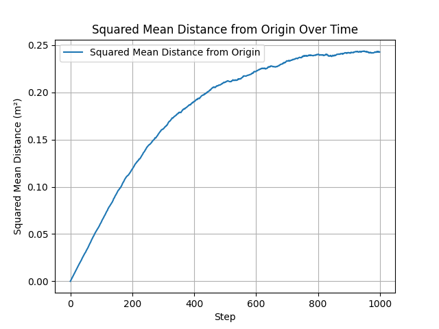
Squared RMS displacement $r_{\text{RMS}}^2$ vs. step number for fixed-step random walks. The linear trend confirms Einstein’s diffusion law $\langle r^2 \rangle = 6Dt$ in the free-diffusion regime before particles approach the reflective boundaries.
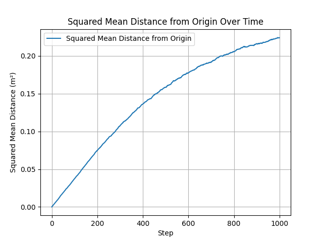
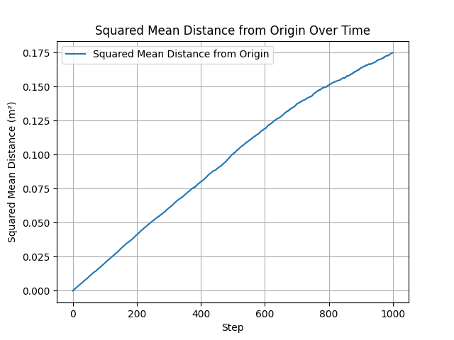
Comparison of different step-length distributions: volumetric (left) and radial (right). All produce the expected linear MSD growth, with differences in the effective diffusion coefficient $D$ arising from the mean squared step length.
Build & Run
Prerequisites
- C++17 compatible compiler (
clang++org++) - OpenMP (via Homebrew:
brew install libompon macOS) - zlib (for
.npzcompression) - Python 3 with
numpy,matplotlib, andffmpeg(for animation export)
Build
# Optimized release build (recommended)
make release

# Debug build (full warnings, no optimization, no OpenMP)
make debug

# Profile-guided optimization (two-step)
make profile-gen && ./bin/main && make profile-use
Run
./bin/main
Visualize
python3 plotting.py
Simulation Parameters
Configured in main.cpp:
| Parameter | Default | Description |
|---|---|---|
movementRadius |
0.025 m | Fixed step length per random walk move |
cubeSize |
1.0 m | Side length of the confining cubic volume |
steps |
5 | Number of time steps simulated |
numPoints |
2500 | Number of independent diffusing particles |
outputFilename |
"output/defusion_output" |
Base path for output files |
Tip: For a clearly visible linear MSD regime before boundary effects dominate, ensure $r_\text{RMS}(t_\text{final}) = \sqrt{6 \cdot \frac{\ell^2}{6} \cdot t_\text{final}} \ll L/2$. With defaults this gives $r_\text{RMS}(5) \approx 0.056\,\text{m}$ against a half-width of $0.5\,\text{m}$ — comfortably in the free-diffusion regime.
Project Structure
Project 6: Defusion/
|-- main.cpp        # Entry point: configures and runs the simulation
|-- processing.h    # Space class: random walk, RMS, CSV and NPZ output
|-- Makefile        # Multi-target build: debug, release, profile-guided
|-- plotting.py     # Python visualization: 3D animation + MSD plot
`-- output/
    |-- defusion_output.npz            # Compressed simulation data
    |-- defusion_output_Positions.csv  # Per-step particle positions (CSV)
    |-- defusion_output_RMS.csv        # Per-step RMS displacement (CSV)
    |-- diffusion_animation.mp4        # Animated 3D particle cloud
    `-- Mean_Squared_Distance_plot.png # MSD vs step number
Key Techniques at a Glance
| Technique | Purpose |
|---|---|
| Uniform sphere sampling via $(\cos\phi, \theta)$ parametrization | Guarantees isotropic, unbiased step directions |
| Fixed step length (fixed-radius walk) | Simplest model of normal Brownian diffusion; $D$ is exactly $\ell^2/6\tau$ |
| Reflective (mirror) boundary conditions | Conserves particle number; models an elastic confining wall |
| Sequential step loop + parallel particle loop | Respects the $t \to t+1$ dependency while fully parallelizing the independent particle dimension |
| Per-thread RNG seeded by thread ID + clock | Thread-safe, uncorrelated random streams without mutexes |
| Parallel CSV row formatting + parallel NPZ flattening | Avoids I/O becoming a serial bottleneck for large particle counts |
std::array<float, 3> in contiguous nested vectors |
Cache-friendly layout aligned with the parallel access pattern |
| NPZ output with self-describing metadata array | Single-file, compressed, self-contained data portable to any NumPy environment |
Nels Buhrley — Computational Physics, 2026