Project 7: The 3D Ising Model
Tip. Every highlighted link in this page is clickable. For fast navagation use Table of Contents
Author: Nels Buhrley
Language: C++17 with OpenMP · Python 3 (visualization)
HPC: Run on the BYU Supercomputer (128 CPUs via SLURM)
Build: make release — see Build & Run
Snapshot
- Built a full 3D Ising-model Monte Carlo engine with checkerboard updates and precomputed energy tables for high-throughput spin-flip evaluation.
- Executed large temperature-field parameter sweeps with OpenMP plus SLURM, scaling runs to 128 CPU cores on BYU HPC infrastructure.
- Generated magnetization surfaces and contour analyses that recover expected critical behavior near the Curie transition.
- Demonstrates strong capability in statistical-physics simulation, performance optimization, and HPC production workflows.
For a fast technical check, jump to Code Structure, Results, and Build & Run.
Table of Contents
- Snapshot
- Overview
- Physics Background
- Code Structure
- Results
- Sources of Error
- Build & Run
- Simulation Parameters
- Key Techniques
- Project Structure
Overview
This project implements a full Monte Carlo simulation of the three-dimensional Ising model on a cubic lattice. The simulation sweeps across a two-dimensional parameter space of temperature $T$ and external magnetic field $h$, producing a surface of average magnetization $\langle m \rangle(T, h)$ that captures the system’s full thermodynamic behavior — including the ferromagnetic phase transition and the onset of spontaneous symmetry breaking.
The implementation combines the Metropolis–Hastings algorithm, a checkerboard (black-red) lattice decomposition, precomputed energy lookup tables, and OpenMP multi-threaded parallelism to efficiently map the parameter space.
Physics Background
The Ising Hamiltonian
The Ising model places discrete binary spins $\sigma_i \in {-1, +1}$ on the sites of a 3D cubic lattice of $N \times N \times N$ sites, with total energy:
\[\mathcal{H} = -J \sum_{\langle i,j \rangle} \sigma_i \sigma_j - h \sum_i \sigma_i\]where $J > 0$ is the ferromagnetic exchange coupling (set to 1 in natural units), the first sum runs over nearest-neighbor pairs (6 per site in 3D), and $h$ is the external magnetic field.
Phase Transition
At low temperature and zero field the system exhibits spontaneous magnetization. As temperature rises, entropy dominates and magnetization collapses continuously to zero at the Curie point $T_c$. The 3D Ising model has:
\[T_c \approx 4.51 \; J/k_B\]in units where $J = k_B = 1$.
Observable: Average Magnetization
The primary output at each $(T, h)$ point is the average magnetization per spin:
\[\langle m \rangle = \frac{1}{N^3} \sum_i \sigma_i\]Code Structure
All simulation logic lives in two files:
| File | Role |
|---|---|
main.cpp |
Sets parameters, constructs Simulation, calls runIsingSimulation() |
processing.h |
Material class (Metropolis engine), Simulation class (sweep, analysis, I/O) |
Material Class
Each Material instance represents one independent lattice at a fixed $(T, h)$ pair.
Construction
Material(int n, float temperature, float magnetization, int numIterations, uint32_t seed)
The physical lattice is $N \times N \times N$ but the internal allocation is $(N+2)^3$ to hold ghost boundary layers. The constructor calls three setup methods in order:
establishRNG()— seeds a per-objectstd::mt19937fromseed, giving each parallel worker its own independent random streaminitializeSpinsRandomly()— fills the inner lattice with random $\pm 1$ values; an overloadinitializeSpinsUniformly(int8_t)sets all spins to a single value insteadprecalculateEnergyTables()— buildsdeltaE_table[2][7]andexp_table[2][7](see Precomputed Tables)
Spins are stored as int8_t in a flat 1D std::vector<int8_t> using row-major indexing:
Using int8_t rather than int keeps the $100^3$ lattice $4\times$ smaller and cache-friendly for the sequential $z$-loop. getSpin() and setSpin() are inlined accessors over this flat array.
Precomputed Energy Lookup Tables
flipSpin() is the innermost function, called $O(N^3 \times \text{iterations})$ times. In a 3D model with 6 neighbors, the neighbor sum $S \in {-6,-4,-2,0,+2,+4,+6}$ admits only 7 values. Combined with the 2 spin states, only 14 distinct $\Delta E$ values ever arise:
precalculateEnergyTables() computes both $\Delta E$ and $e^{-\Delta E/T}$ for all 14 combinations once, before any sweep:
float deltaE_table[2][7];
float exp_table[2][7];
The inner loop then performs a plain array dereference instead of calling exp().
flipSpin(x, y, z) — Metropolis Step
For site $(x,y,z)$, the neighbor sum is computed and mapped to a table index:
void flipSpin(int x, int y, int z) {
    uint8_t neighborstate = (sum of 6 neighbors) / 2 + 3;  // maps [-6,6] -> [0,6]
    uint8_t spinState = (getSpin(x, y, z) + 1) / 2;        // maps {-1,+1} -> {0,1}
    if (deltaE_table[spinState][neighborstate] <= 0 ||
        distribution(gen) < exp_table[spinState][neighborstate]) {
        setSpin(x, y, z, -getSpin(x, y, z));
        currentTotalMagnetization += 2 * getSpin(x, y, z);  // incremental update
    }
}
The Metropolis acceptance rule is satisfied: always flip if $\Delta E \leq 0$, otherwise flip with probability $e^{-\Delta E/T}$. When a flip occurs, currentTotalMagnetization is updated by $\pm 2$ rather than recomputed — avoiding an $O(N^3)$ sum every step.
iteration() — One Full Lattice Sweep
Each call performs three stages.
Stage 1 — Ghost layer refresh (periodic boundary conditions):
Rather than wrapping indices on every neighbor access, the $(N+2)^3$ lattice carries one ghost cell on each face. Before each sweep all six faces are refreshed by copying the opposite interior face:
// Z faces
for (x) for (y) {
    setSpin(x, y, 0,   getSpin(x, y, n-2));   // bottom ghost <- top interior
    setSpin(x, y, n-1, getSpin(x, y, 1));     // top ghost <- bottom interior
}
// Y and X faces updated the same way
This is $O(N^2)$ per sweep, negligible against the $O(N^3)$ spin work, and keeps the inner loop branch-free.
Stage 2 — Black pass (sites where $(x+y+z)$ is even):
for (x = 1; x < n-1; x++)
    for (y = 1; y < n-1; y++)
        for (z = (x+y)%2 + 1; z < n-1; z += 2)
            flipSpin(x, y, z);
Stage 3 — Red pass (sites where $(x+y+z)$ is odd):
for (x = 1; x < n-1; x++)
    for (y = 1; y < n-1; y++)
        for (z = (x+y+1)%2 + 1; z < n-1; z += 2)
            flipSpin(x, y, z);
The parity offset (x+y)%2 selects the correct starting $z$ so every visited site satisfies the desired color. Striding by 2 ensures no two sites in the same pass share a neighbor, making all updates within a pass conflict-free. A black pass followed by a red pass constitutes one full Monte Carlo sweep.
runSimulation() and MagneticSusceptibility()
runSimulation() runs in two phases:
Phase 1 — Burn-in (5 * n sweeps):
for (int i = 0; i < 5 * n; i++) iteration();
These sweeps allow the system to reach thermal equilibrium from its initial state without contributing to any observable. The initial spin state (random or uniform) is forgotten here.
Phase 2 — Measurement (numIterations sweeps):
for (int i = 0; i < numIterations; i++) {
    iteration();
    float m = (float)currentTotalMagnetization / N;
    sum_magnetization        += m;
    sum_magnetization_squared += m * m;
    sum_abs_magnetization    += std::abs(m);
}
averageAbsMagnetization     = sum_abs_magnetization     / numIterations;
averagemagnetization        = sum_magnetization          / numIterations;
averageMagnetizationSquared = sum_magnetization_squared  / numIterations;
After each sweep, the instantaneous magnetization per spin $m = M_\text{total}/N^3$ is read from currentTotalMagnetization (maintained incrementally by flipSpin) — no full-lattice sum is needed. Three accumulators are kept to compute $\langle m \rangle$, $\langle \vert m \vert \rangle$, and $\langle m^2 \rangle$.
MagneticSusceptibility() is called after the simulation completes and derives $\chi$ from the variance of $\vert m\vert $:
Using $\langle \vert m\vert \rangle$ rather than $\langle m \rangle^2$ avoids cancellation errors in symmetry-broken phases where positive and negative magnetization states are sampled equally, which would drive $\langle m \rangle \to 0$ even deep in the ferromagnetic phase.
Simulation Class
The Simulation class owns the full parameter sweep, analysis, and output. main.cpp constructs one instance and calls runIsingSimulation(), which chains three methods:
Simulation::runIsingSimulation()
    |-- runSimulation()                       -- parallel Metropolis sweep
    |-- findCriticalTemperatureAndCalculateBeta()  -- post-process
    `-- saveResults()                         -- NPZ + CSV output
Simulation::runSimulation() — Parallel Sweep
1. Generate a unique seed for every (h, T) pair from a master RNG
2. #pragma omp parallel for collapse(2) schedule(dynamic)
      for each (T[i], h[j]):
          Material material(n, T[i], h[j], iterations, +1, seed[j][i])
          material.runSimulation()
          avg_magnetizations[j][i]       = material.averageMagnetization
          magnetic_susceptibilities[j][i] = material.magneticSusceptibility
Each Material is initialized with all spins uniformly $+1$ (via the second constructor overload), which biases the system into the ferromagnetic minimum and reduces equilibration time. Seeds are drawn from a 2D array populated by a single-threaded master RNG before the parallel region, eliminating data races on the generator state.
findCriticalTemperatureAndCalculateBeta() — Critical Analysis
This runs in a second OpenMP parallel loop over field rows j:
Step 1 — Find $T_c$: The critical temperature for each $h$ value is identified as the temperature where $\chi(T)$ is maximum:
for (i in 0..numTempSteps)
    if (magnetic_susceptibilities[j][i] > maxSusceptibility)
        criticalTempIndex = i;
critical_temperatures[j] = temperatures[criticalTempIndex];
This works because $\chi$ diverges (and in a finite system peaks sharply) at $T_c$.
Step 2 — Fit $\beta$: Near $T_c$ the order parameter scales as $\langle \vert m\vert \rangle \sim (T_c - T)^\beta$. Taking logs gives: \(\ln \langle \vert m\vert \rangle = \beta \ln(T_c - T) + \text{const}\) The code selects up to 40 points just below $T_c$ (filtering out points where $\vert m\vert < 0.01$ or $T \geq T_c$ to avoid log-of-zero issues) and fits the slope via ordinary least squares in log-log space:
double numerator = n * sumLogMLogT - sumLogM * sumLogT;
double denominator = n * sumLogTSquared - sumLogT * sumLogT;
double slope = numerator / denominator;
beta_exponents[j] = slope;
The extracted $\beta$ is saved alongside $T_c$ for each field row.
Results
Magnetization Surface
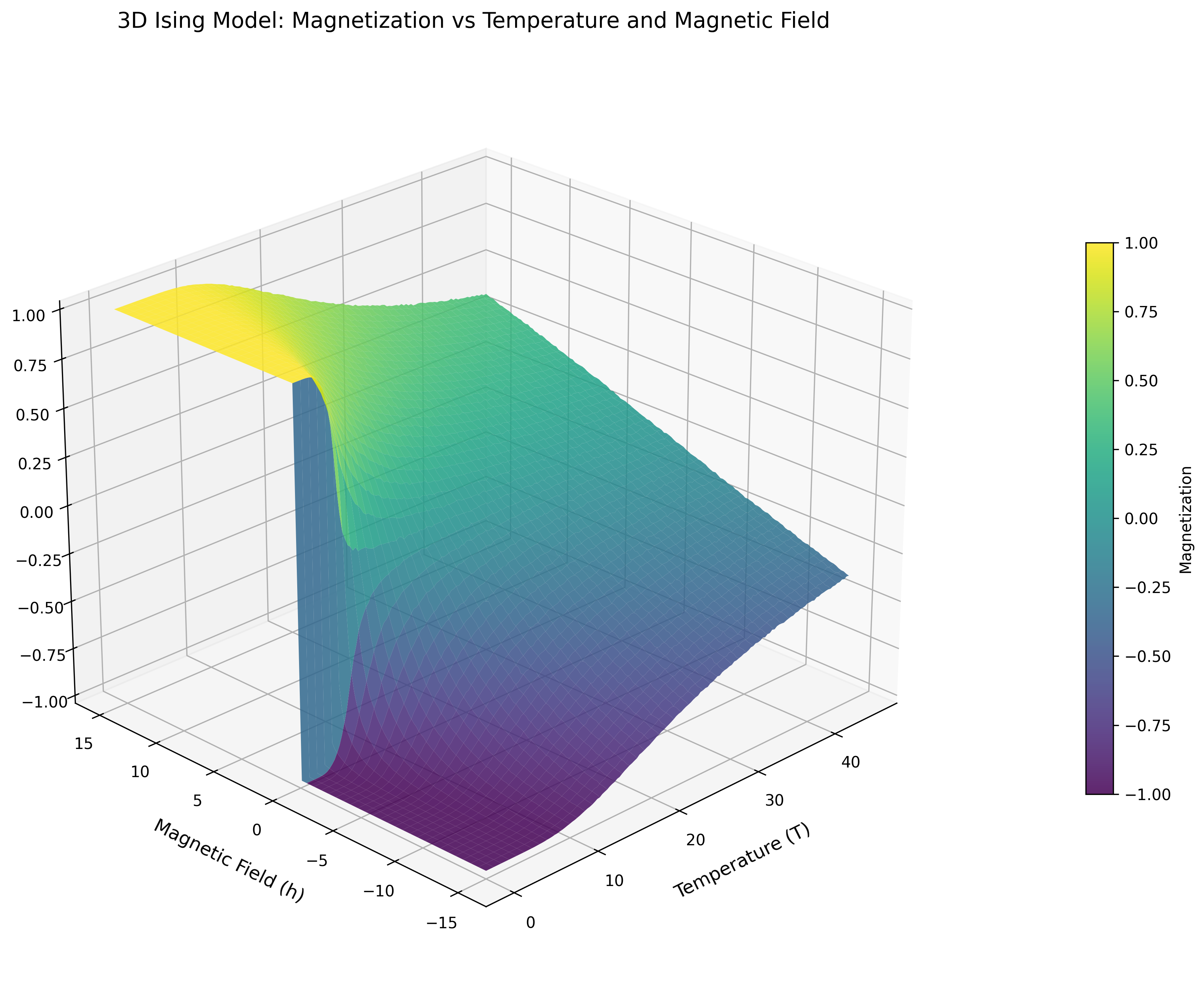
3D surface plot of the average magnetization $\langle m \rangle(T, h)$. The sharp cliff at $T_c \approx 4.51\,J/k_B$ (at $h = 0$) marks the ferromagnetic phase transition — the system transitions from ordered (magnetized) to disordered (paramagnetic) as temperature rises.
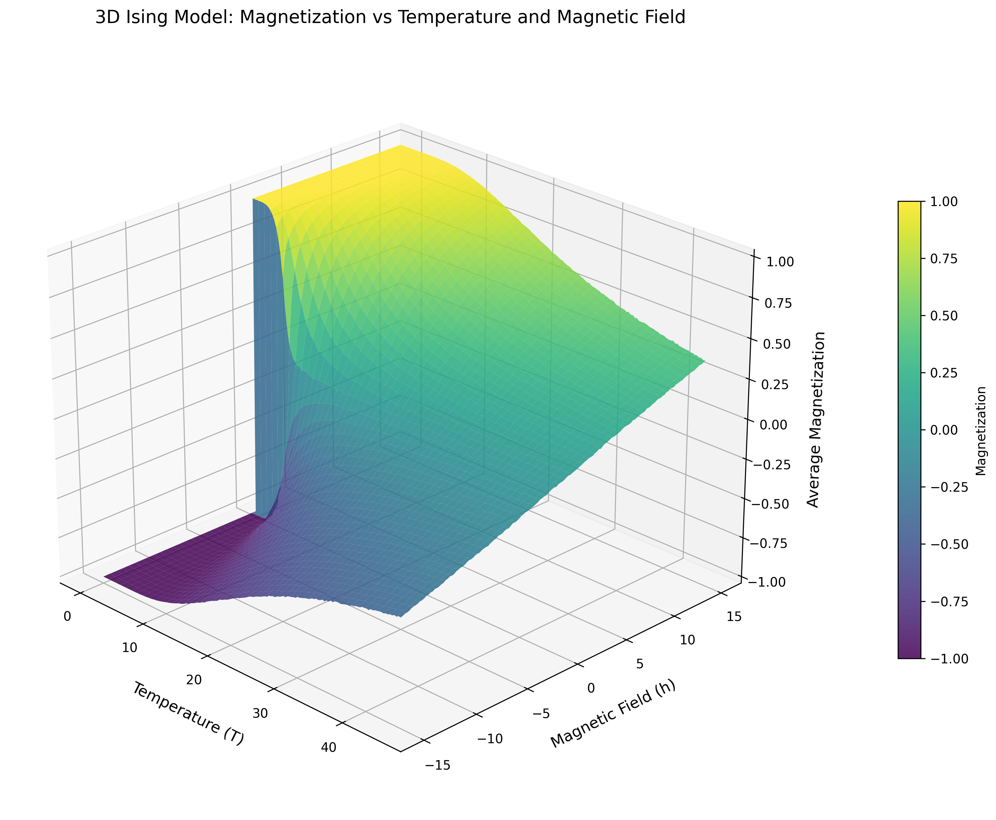
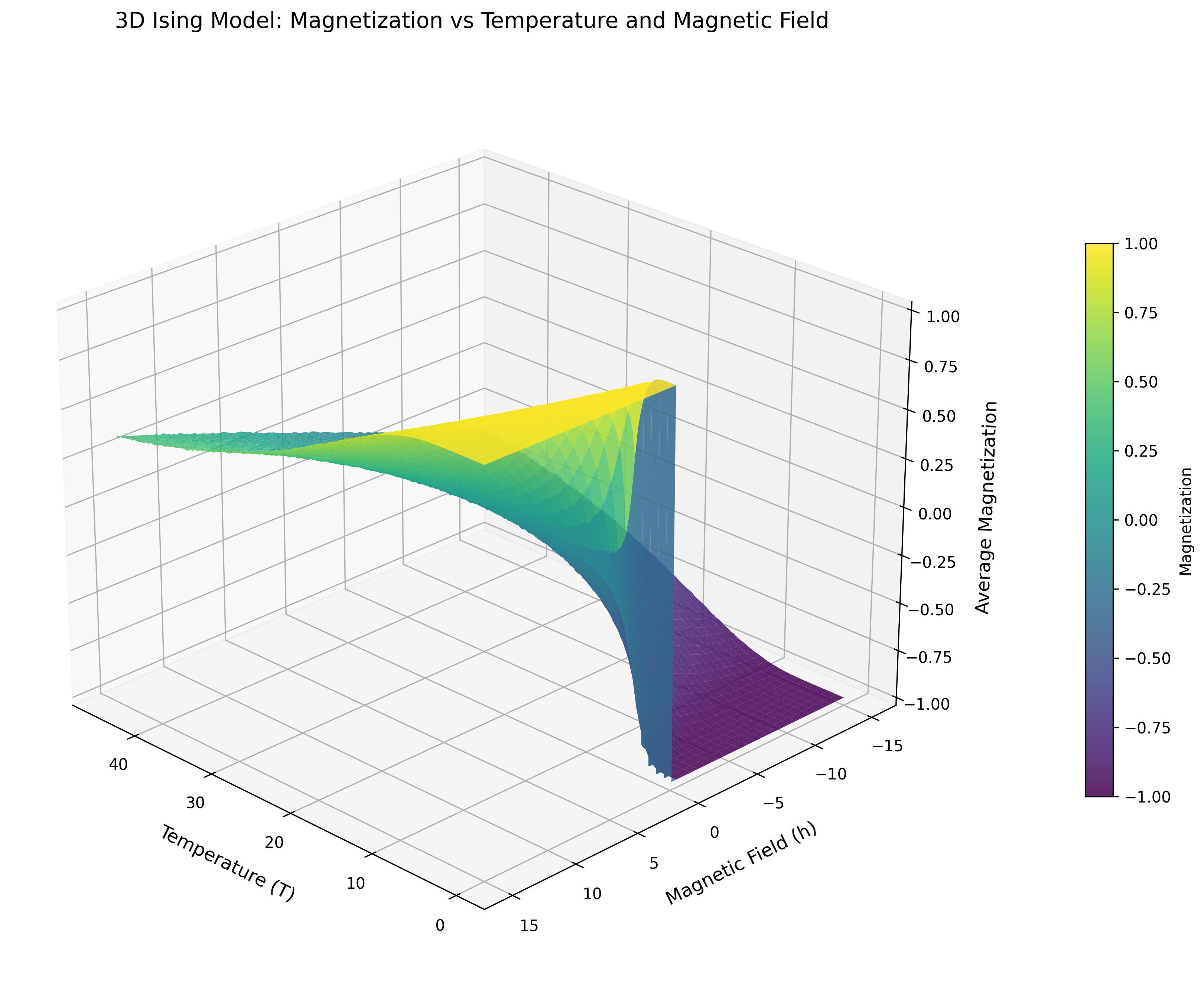
Alternative viewing angles of the magnetization surface, showing the symmetry-breaking structure: for $h > 0$ the system prefers $+m$, for $h < 0$ it prefers $-m$, and the transition sharpens as $h \to 0$.
Magnetization Contour Map
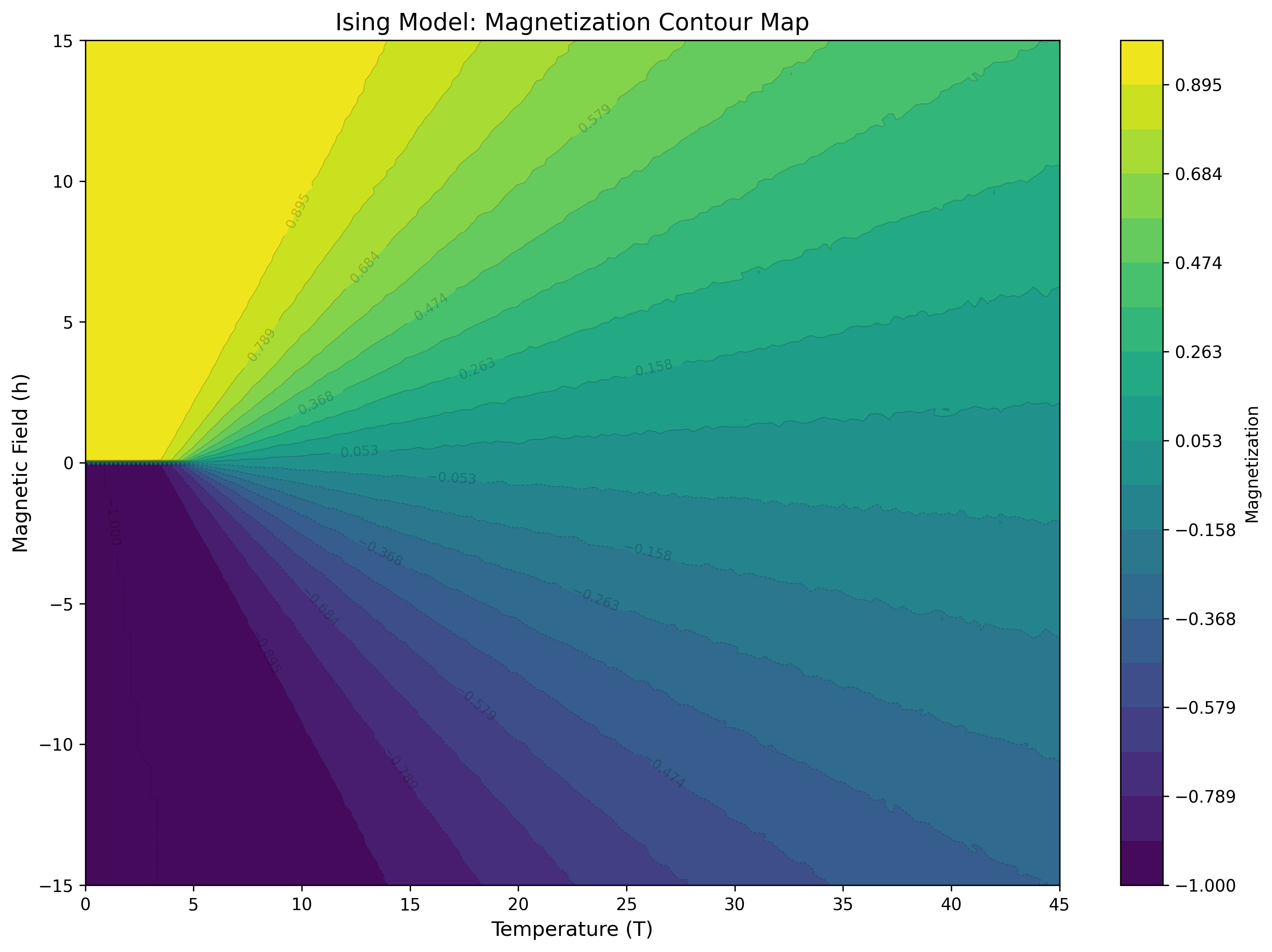
Contour plot of $\langle m \rangle$ in the $(T, h)$ plane. The critical temperature is visible as the boundary between the ordered (yellow/purple) and disordered (color gradiant) phases.
Magnetization vs. Temperature
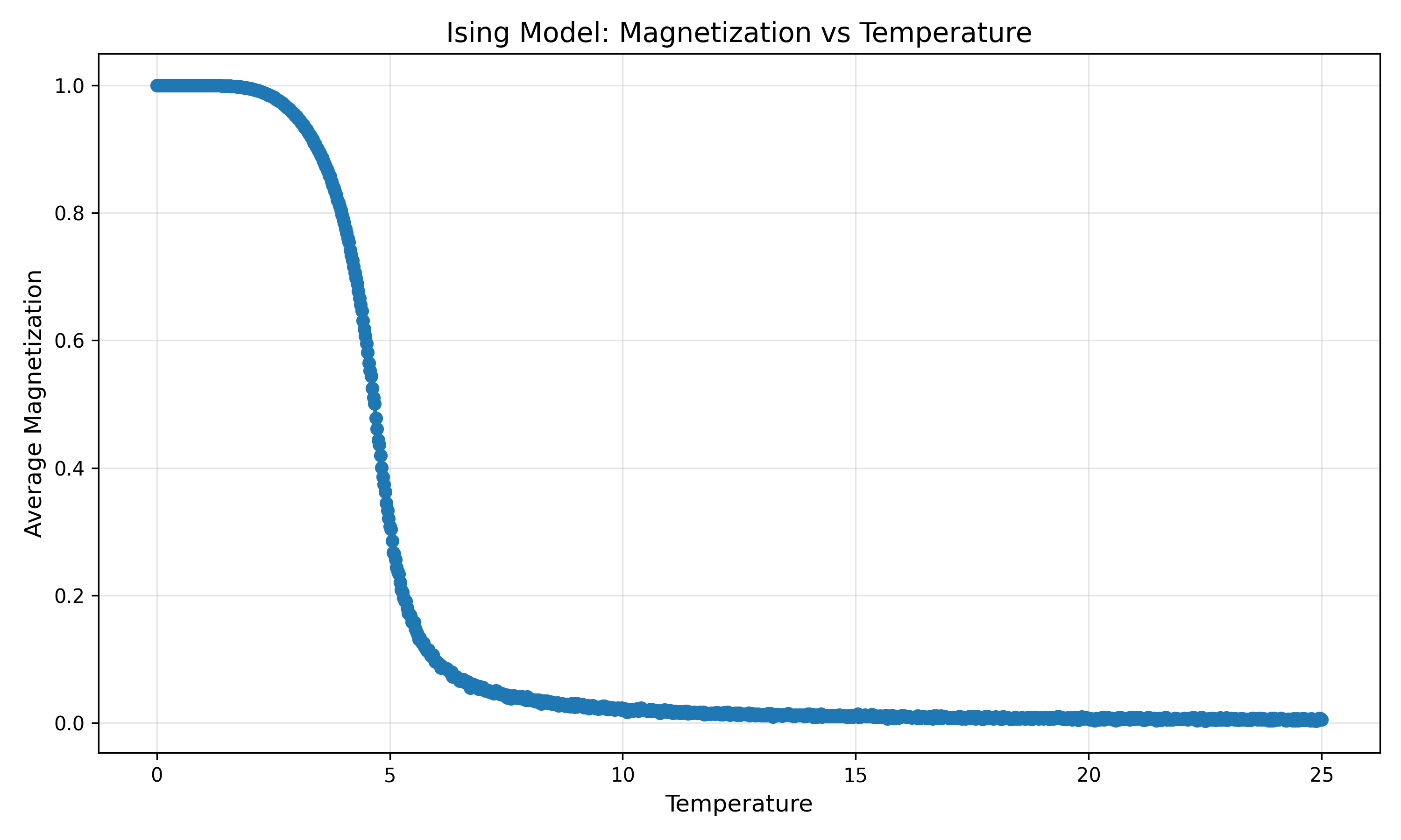
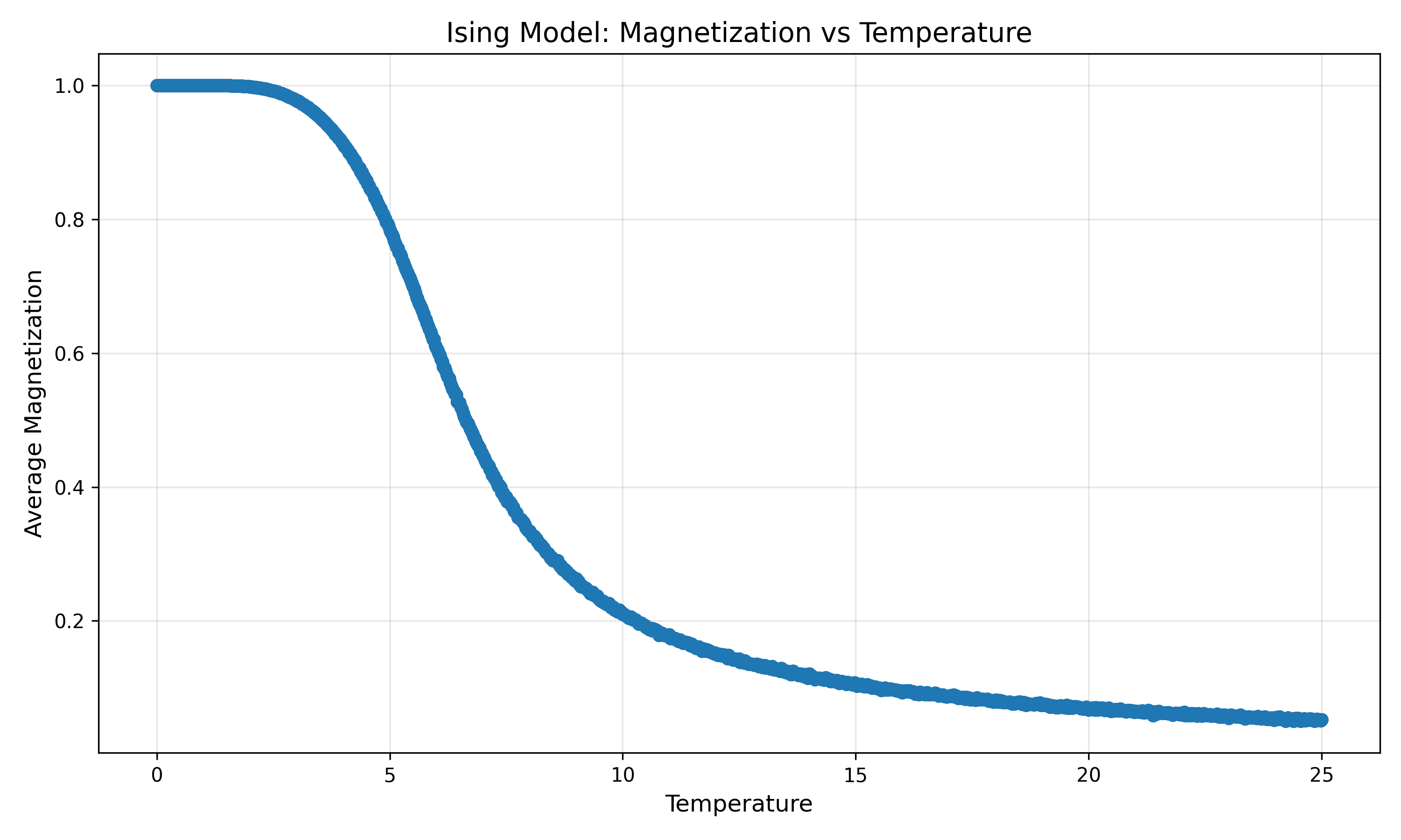
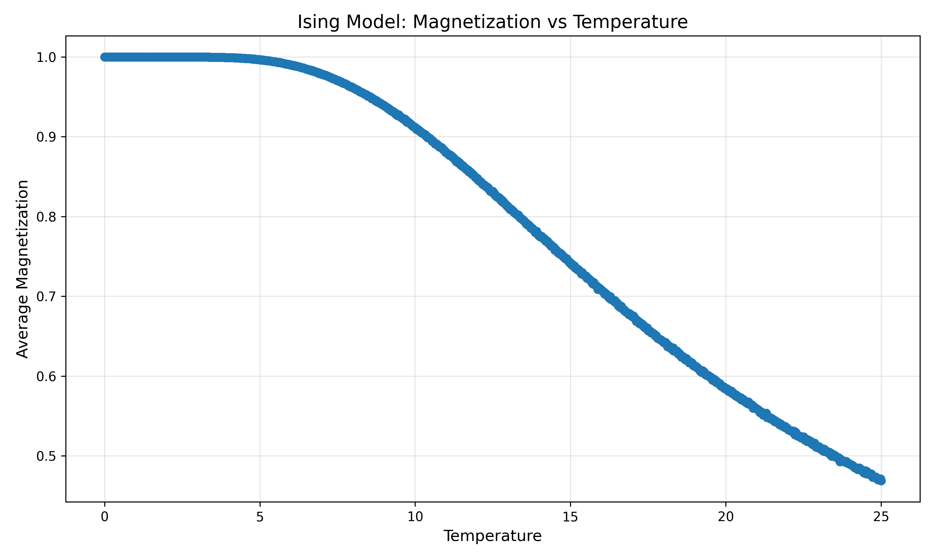
Magnetization as a function of temperature at three field strengths. At weak field ($h = 0.1$), the transition is sharp. Increasing $h$ smooths the transition and shifts the effective crossover temperature — at strong field ($h = 10$), magnetization persists well above $T_c$.
Interactive 3D Visualization
The interactive plot above renders the same 3D field as the static slice, but with full rotational control. You can:
- Rotate the 3D volume by dragging your mouse to inspect the potential structure from any angle
- Zoom using the scroll wheel to examine fine details
This allows intuitive exploration of the phase change geometry without generating dozens of static images.
Sources of Error
| Source | Nature | Mitigation |
|---|---|---|
| Statistical fluctuations | MC results are stochastic | Increase iterations; ensemble-average over seeds |
| Finite-size effects | Finite $N$ smears the transition; $T_c(N) \neq T_c(\infty)$ | Increase $N$; apply finite-size scaling |
| Equilibration error | Early sweeps retain memory of the initial state | 100-sweep burn-in is hardcoded in runSimulation(); increase for larger $N$ |
| Parameter discretization | $T$ and $h$ sampled on finite grids | Increase tempSteps/numHSteps near $T_c$ |
Computational complexity (per $(T,h)$ point): $\mathcal{O}(N^3 \times \text{iterations})$
Total: $\mathcal{O}(N^3 \times \text{iterations} \times N_T \times N_h)$ — roughly $8 \times 10^{10}$ spin-update operations at default parameters.
Build & Run
Prerequisites
- C++17 compiler (
g++orclang++) - OpenMP (
brew install libompon macOS) - zlib (for
.npzoutput) - Python 3 with
numpyandmatplotlib
Build Targets
make release   # Optimized build (-O3, LTO, vectorization, march=native)
make unsafe    # Adds -ffast-math (may introduce minor FP drift)
make debug     # -O0, full warnings, OpenMP disabled
make profile-gen && ./bin/main && make profile-use  # Profile-guided optimization
Run
./bin/main
Output is saved to output/ising_results.npz and output/ising_results.csv:
| Array | Shape | Description |
|---|---|---|
avg_magnetization |
(N_h, N_T) |
$\langle m \rangle$ at each $(h, T)$ |
magnetic_susceptibility |
(N_h, N_T) |
$\chi$ at each $(h, T)$ |
temperatures |
(N_T,) |
Temperature grid |
magnetic_fields |
(N_h,) |
Magnetic field grid |
critical_temperatures |
(N_h,) |
$T_c(h)$ — peak susceptibility per field row |
beta_exponents |
(N_h,) |
Fitted $\beta$ exponent per field row |
Visualize
python3 plotting.py
Produces 3D surface plots and a 2D contour map in output/.
Simulation Parameters
Configured in main.cpp:
| Parameter | Default | Description |
|---|---|---|
N |
100 | Cubic lattice edge length ($N^3$ spins) |
iterations |
200 | MC sweeps per $(T, h)$ point |
minTemp / maxTemp |
0 – 45 | Temperature range ($J/k_B$) |
tempSteps |
200 | Temperature grid points |
hMin / hMax |
−15 – +15 | External field range |
numHSteps |
200 | Field grid points |
Key Techniques
| Technique | Purpose |
|---|---|
| Metropolis–Hastings MCMC | Correct Boltzmann sampling |
| Precomputed $\Delta E$ and $e^{-\Delta E/T}$ tables | Eliminates exp() from the inner loop |
| Checkerboard (black-red) decomposition | Race-free simultaneous updates within a sweep |
| Ghost boundary layers | Branch-free periodic boundary enforcement |
int8_t + flat 1D array |
$4\times$ smaller than int; cache-friendly $z$-loop |
| Incremental magnetization tracking | $O(1)$ magnetization update per flip instead of $O(N^3)$ |
| 100-sweep burn-in | Discards initial transient before measuring observables |
| Running accumulators for $\langle m \rangle$, $\langle \vert m\vert \rangle$, $\langle m^2 \rangle$ | Enables susceptibility and critical-exponent analysis |
| Peak susceptibility $\to T_c$ | Locates the critical temperature per field row |
| Log-log OLS regression $\to \beta$ | Extracts the critical exponent from magnetization scaling below $T_c$ |
collapse(2) + dynamic scheduling |
Scalable multi-core parallelism across $(T, h)$ |
| Per-thread Mersenne Twister | Statistically independent, uncorrelated random streams |
| Profile-guided optimization (PGO) | Compiler uses runtime data for branch prediction and inlining |
Project Structure
Project 7: The Ising Model/
|-- main.cpp        # Entry point: configures and launches the simulation
|-- processing.h    # Material + Simulation classes: Metropolis engine, sweep, analysis, I/O
|-- Makefile        # Multi-target build: debug, release, unsafe, profile-guided
|-- plotting.py     # Python visualization: 3D surface plots + contour map
|-- job.sh          # SLURM batch script (BYU Supercomputer -- 128 CPUs, 1 hr)
|-- requirements.txt
|-- slurm_out/      # SLURM stderr logs from HPC runs
|   |-- slurm_10498461.err
|   |-- slurm_10498501.err
|   |-- slurm_10537695.err
|   |-- slurm_10537987.err
|   `-- slurm_10538011.err
`-- output/
    |-- Out_1/                              # Simulation run 1 (Best Visuals)
    |   |-- magnetization_3d_surface_angle1--4.png
    |   |-- magnetization_contour.png
    |   `-- notes.md
    |-- Out_2/                              # Simulation run 2 (Finest Mesh)
    |   |-- ising_results.npz
    |   |-- magnetization_3d_surface_angle1--4.png
    |   |-- magnetization_contour.png
    |   `-- notes.md
    |-- Out_3/                              # Simulation run 3 (most recent full output)
    |   |-- ising_results.npz              # Compressed simulation data (NumPy)
    |   |-- ising_results.csv              # Magnetization + susceptibility (CSV)
    |   |-- magnetization_3d_surface_angle1--4.png
    |   |-- magnetization_contour.png      # 2D contour map M(T,h)
    |   `-- notes.md
    |-- Magnetization Vs. Temperture at destinct H values/
    |   |-- magnetization_vs_temperature_h=0.1.png
    |   |-- magnetization_vs_temperature_h=1.png
    |   `-- magnetization_vs_temperature_h=10.png
    `-- Testing Output/                    # Small test run
        |-- ising_results.npz
        |-- magnetization_3d_surface.png
        `-- magnetization_contour.png
Nels Buhrley — Computational Physics, 2026